When Vision Speaks for Sound

Source-first digest for monthly 2026_05 rank 18, rank_id p017.

Routing status: success
PDF extraction: not used

Motivation / Background

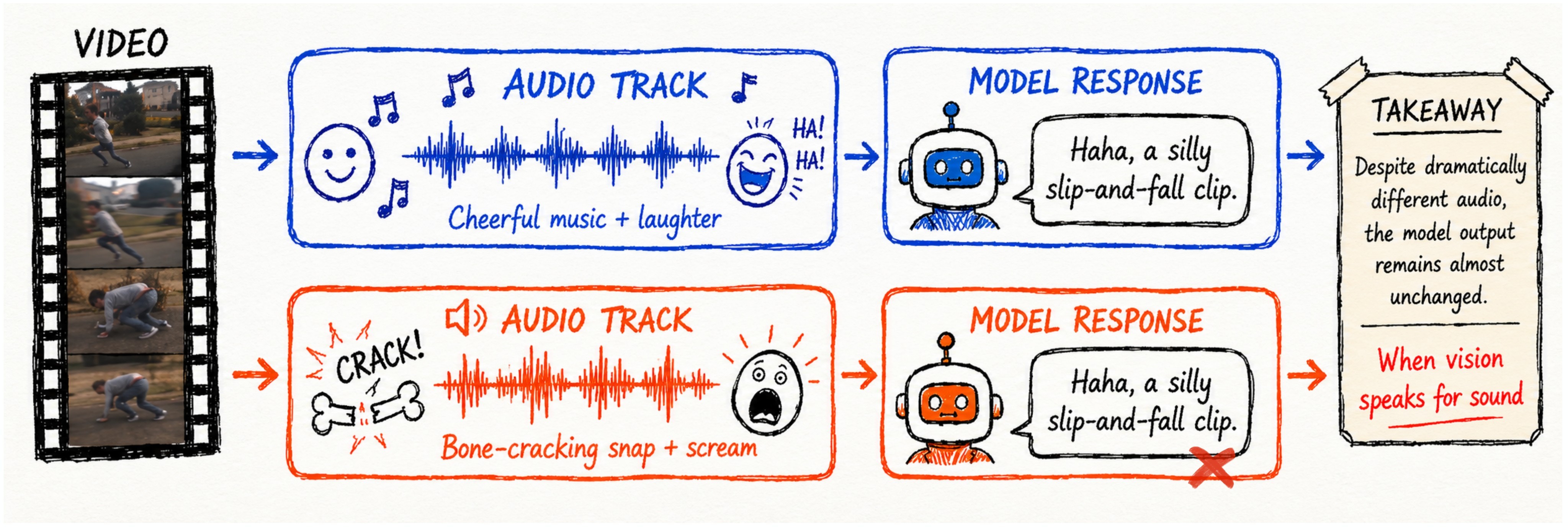
The paper asks whether video-capable multimodal models are actually using audio, or merely inferring what the audio should be from the visual scene. The central failure mode is an audio-visual Clever Hans effect: a model looks audio-grounded because it describes plausible sounds, but the explanation is driven by visual priors rather than verified acoustic evidence.

The authors argue that ordinary audio-video benchmarks hide this shortcut because they preserve natural correlations: barking dogs bark, falling objects make impacts, and speaking faces contain speech. The motivating example in Figure 1 shows why this matters: if the same visible action receives nearly the same sound caption under different audio tracks, the model is not checking the audio stream.

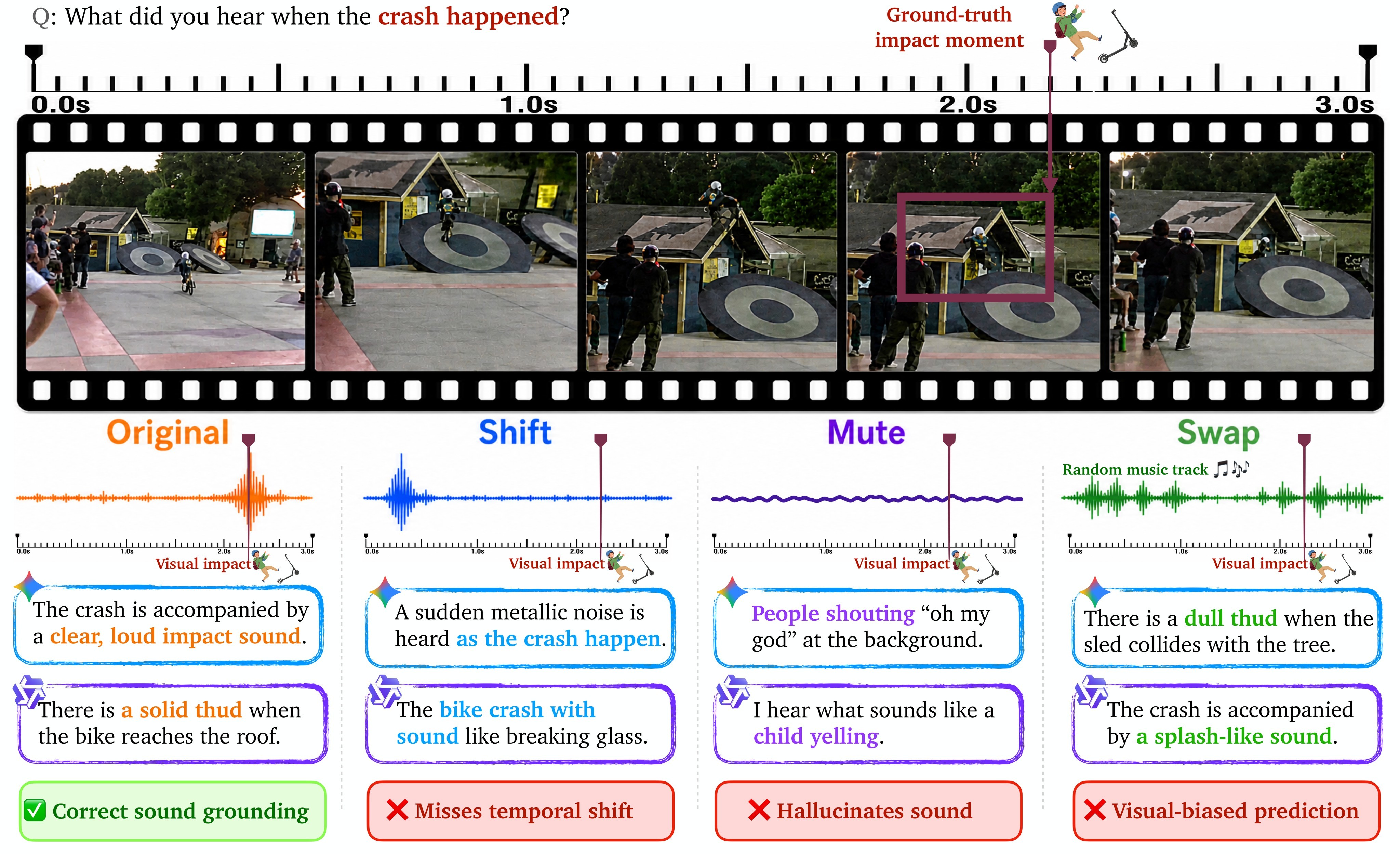
Figure 1. Motivation: visually similar events can drive nearly identical sound captions despite audio-track changes. — **Figure 1. Motivation.** The paper's front-page example frames the core diagnostic problem: the visible event can dominate the answer even when the audio evidence changes.

The proposed diagnostic is Thud: Temporal and Hallucination Unmasking Diagnostics. It builds counterfactual videos that deliberately break audio-visual correlations along three dimensions - temporal synchronization, sound existence, and sound-source consistency. The representative failures in Figure 2 show that Gemini and Qwen3-Omni can still answer from plausible visual acoustics rather than from the actual soundtrack.

Figure 2. Representative Shift, Mute, and Swap failure cases. — **Figure 2. Representative failures.** Shift, Mute, and Swap examples expose missed temporal offsets, hallucinated sounds, and visually biased source matching.

The claim map in Table 1 summarizes the digest's reading of the paper and links each claim to concrete evidence anchors.

Claims And Evidence

Support scores are support-from-paper scores, not independent reproduction scores. A score of 5 means the claim is directly backed by the paper's source text, equations, tables, or figures. A score of 4 means the paper reports direct evidence, but the evidence depends on the authors' benchmark, model interface, or judge setup. A score of 3 means the claim is plausible and source-supported but partly limited, forward-looking, or under-studied.

Claim id	Main claim	Support	Evidence anchors
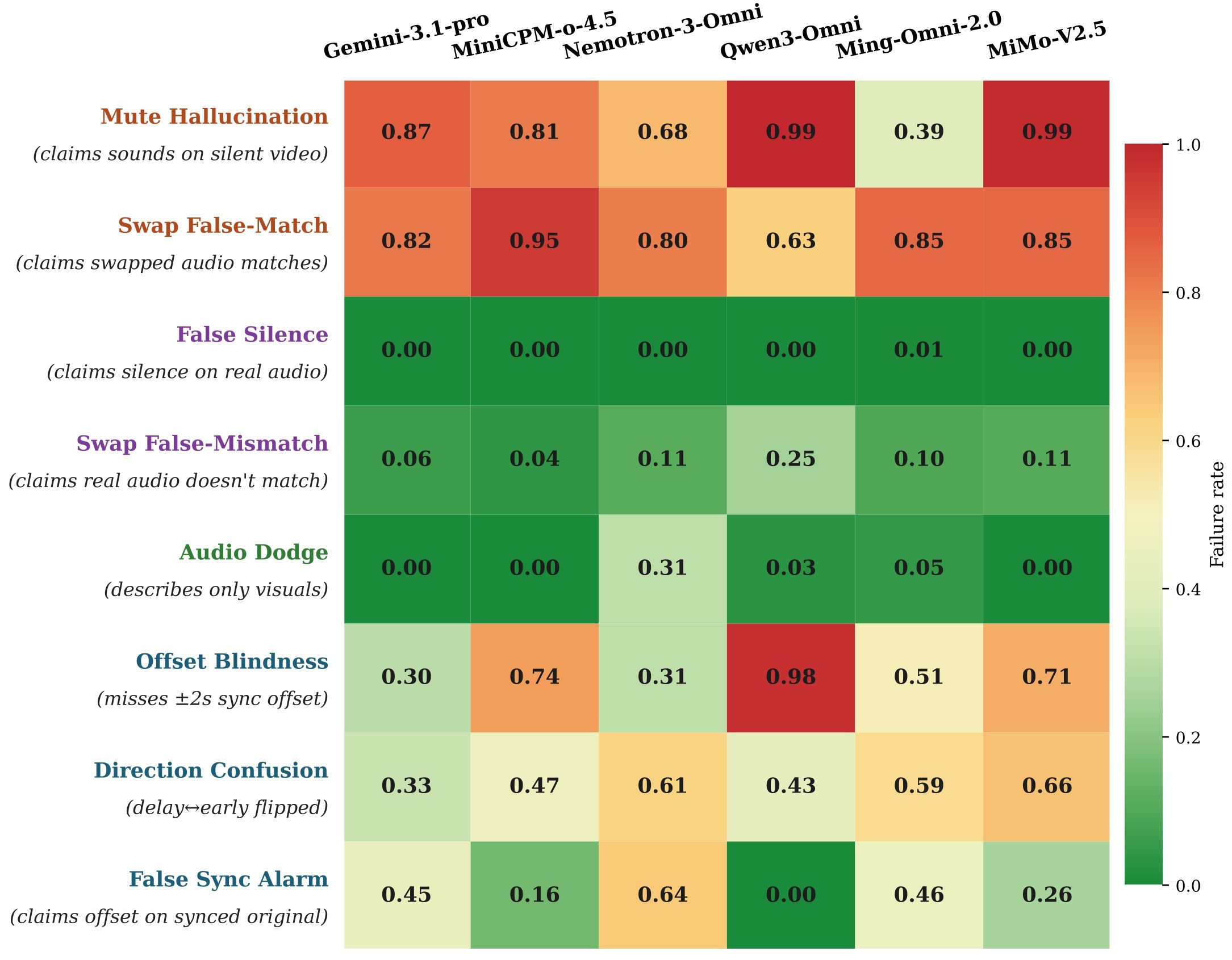
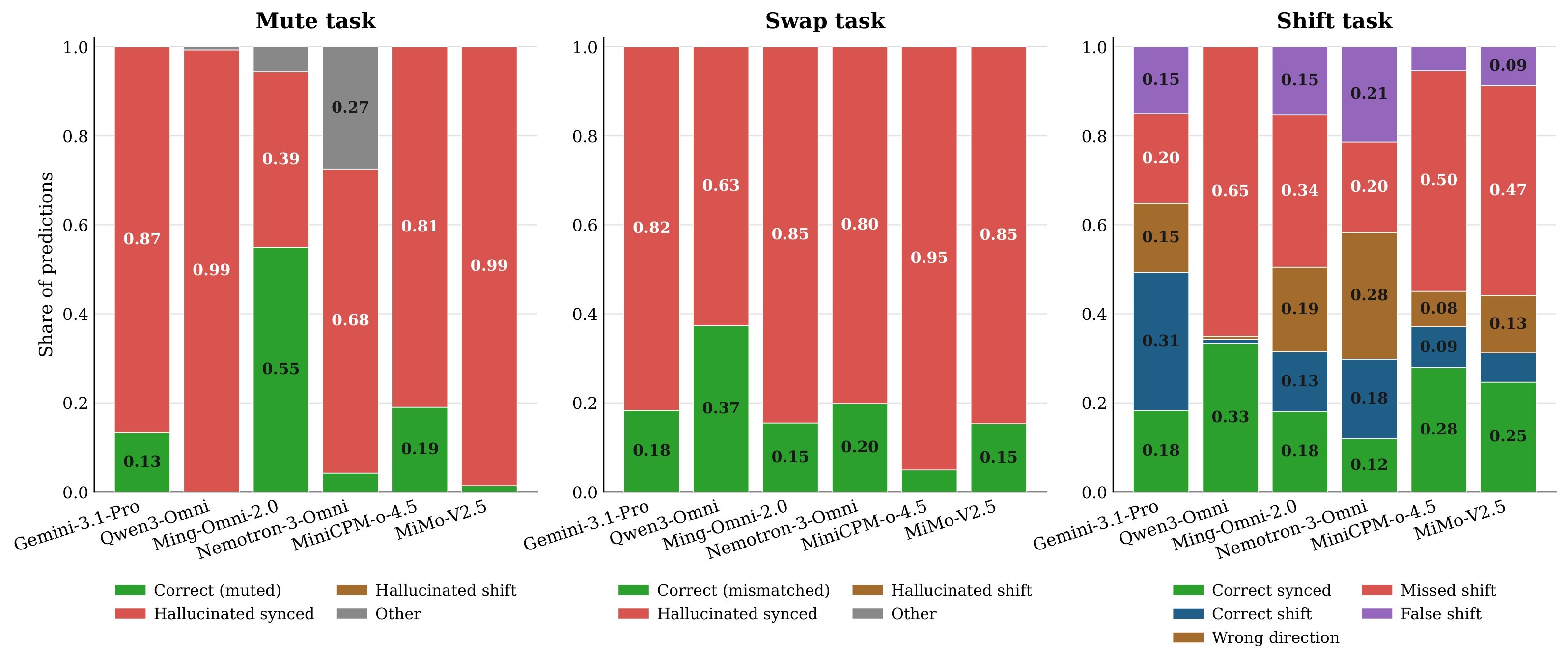
C1	Current video-capable MLLMs often substitute visual-semantic priors for audio verification, creating an audio-visual Clever Hans effect.	5	problem framing, diagnostic results, Table 3, Figure 5, Figure 6
C2	Thud decomposes audio-visual grounding into three counterfactual tests: Shift for timing, Mute for sound existence, and Swap for source consistency.	5	Thud framing, intervention mechanics, key equations, Table 2
C3	The training data pipeline converts verified event-time annotations into chosen/rejected preference pairs where chosen answers check audio evidence and rejected answers encode shortcut-prone responses.	4	annotation pipeline, Figure 3, Figure 4
C4	Across evaluated open and closed models, high accuracy on original videos collapses under counterfactual audio edits.	5	experiment setup, diagnostic results, Table 3, Figure 5, Figure 6
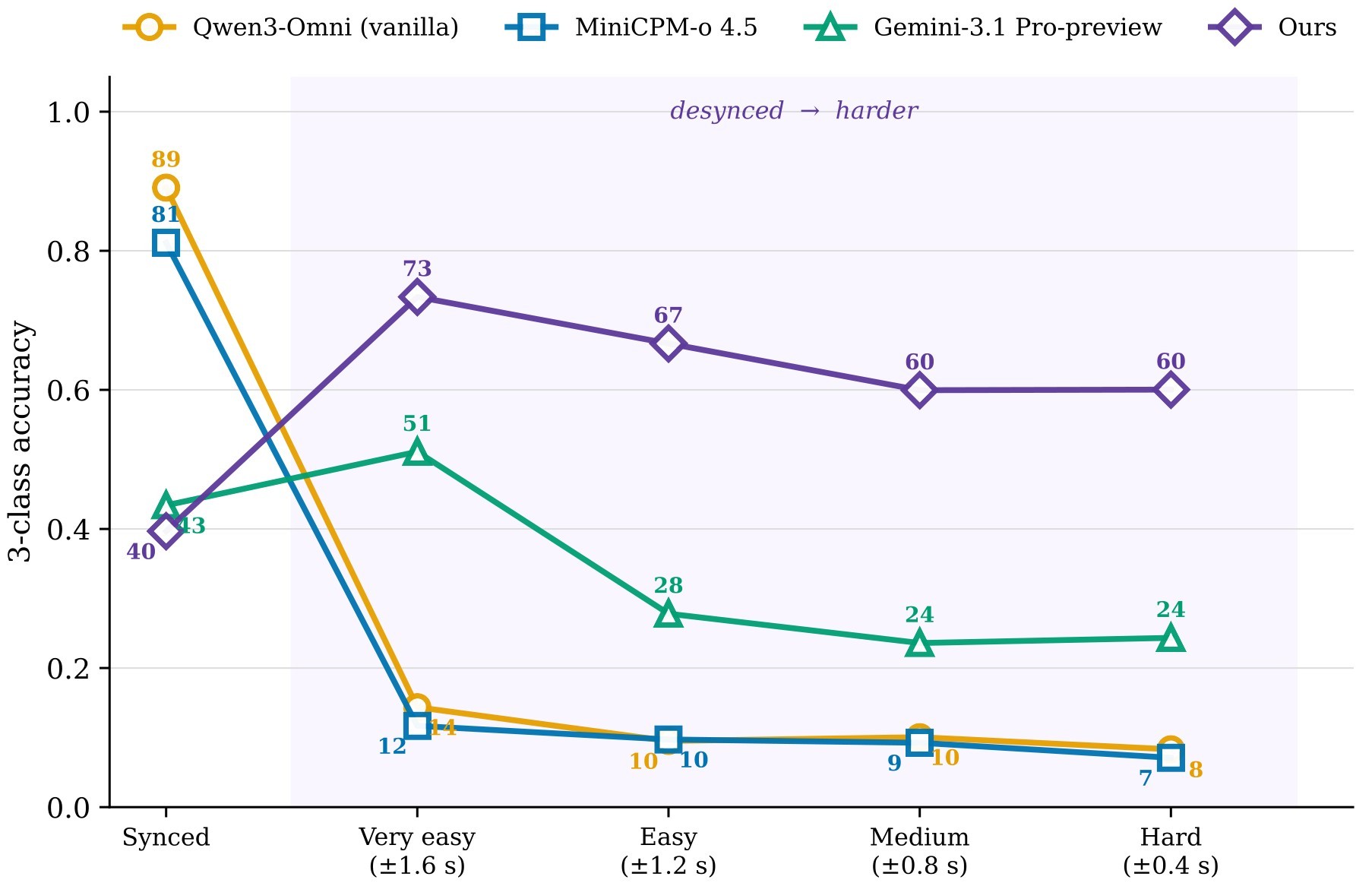
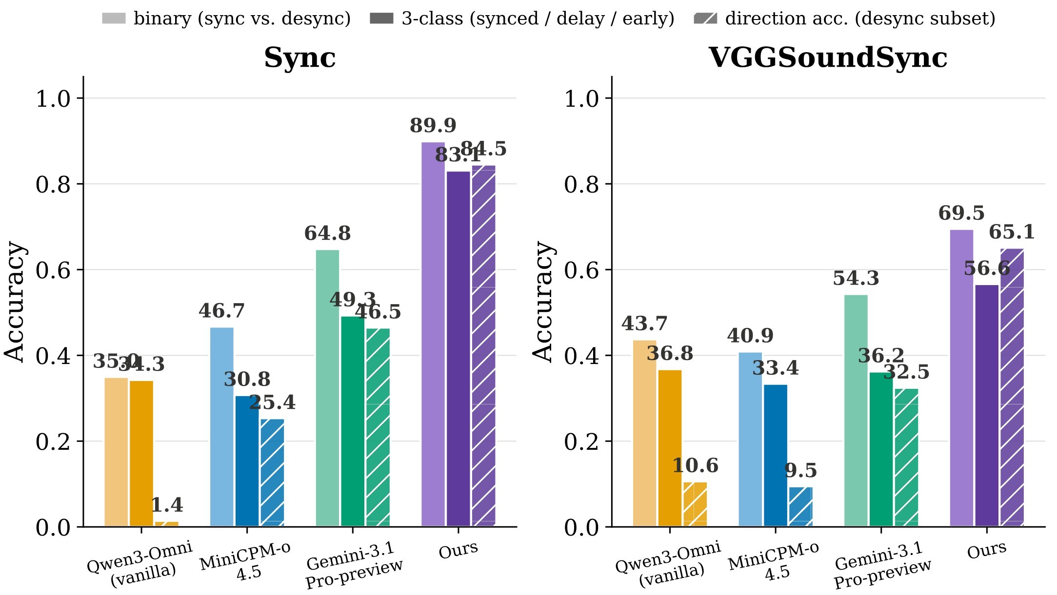
C5	A 10K DPO recipe combining counterfactual temporal preferences with general video preferences improves temporal grounding while preserving general video capability.	4	alignment method, alignment results, Table 4, Figure 7, Figure 8
C6	Extending the recipe with Mute/Swap supervision improves non-temporal intervention performance, but full Mute/Swap training remains less complete than the temporal study.	3	beyond temporal, Figure 9, Figure 10, limitations
C7	Counterfactual audio interventions are best treated as a diagnostic and training stress test, not as a deployment guarantee.	4	limitations, practical takeaways

Core Technical Idea

The core idea is to keep the visual stream fixed while changing the audio stream in a physically interpretable way. Natural videos are useful precisely because they create strong expectations about sound; Thud then breaks those expectations to check whether a model verifies the audio. Table 2 condenses the three tests.

Intervention	Operation	Broken correlation	Diagnostic question
Shift	\(a_{1:T} \rightarrow a_{1:T}^{+\Delta}\)	Temporal synchrony	Is the sound synchronized with the visible event?
Mute	\(a_{1:T} \rightarrow \varnothing\)	Sound existence	Is any sound actually present?
Swap	\(a_{1:T} \rightarrow a'_{1:T}\)	Source consistency	Does the heard sound match the visible event?

The intervention family is defined as:

\tilde{v} = \mathcal{I}_{k}(v), \quad k \in \{\textsc{Shift}, \textsc{Mute}, \textsc{Swap}\}.

For temporal checks:

\mathcal{I}_{\textsc{Shift}}(v;\Delta) = (x_{1:T}, a_{1:T}^{+\Delta}), \quad \Delta \in [-\Delta_{\max}, \Delta_{\max}].

For sound-existence checks:

\mathcal{I}_{\textsc{Mute}}(v) = (x_{1:T}, \varnothing).

For source-consistency checks:

\mathcal{I}_{\textsc{Swap}}(v, v') = (x_{1:T}, a'_{1:T}), \qquad v' = (x'_{1:T}, a'_{1:T}).

The authors also preserve event-level labels:

$$ z_i = (e_i^v, t_i^v, e_i^a, t_i^a), $$

where the visual event/time and acoustic event/time are verified separately. Those labels become preference data:

\mathcal{D}_{\mathrm{pref}} = \left\{ \left( \tilde{v}_i, q_i, y_i^+, y_i^- \right) \right\}_{i=1}^{N}.

Finally, the diagnostic gap used in the appendix averages the accuracy drop from original controls to intervened cases:

\Delta_{\mathrm{shortcut}} = \frac{1}{|\mathcal{D}|} \sum_{d \in \mathcal{D}} \left( \mathrm{Acc}_{\mathrm{Orig},d} - \mathrm{Acc}_{\mathrm{Interv},d} \right), \quad \mathcal{D}=\{\mathrm{Sync}, \mathrm{Exist.}, \mathrm{Consist.}\}.

Method Details

The data construction pipeline in Figure 3 starts from Oops videos because they contain salient acoustic events such as falls, crashes, collisions, and breakage. Gemini provides initial audio-visual event annotations because it can ingest video with audio. GPT and Claude verify visual timestamps over temporally ordered frame units, while human inspection verifies acoustic timestamps.

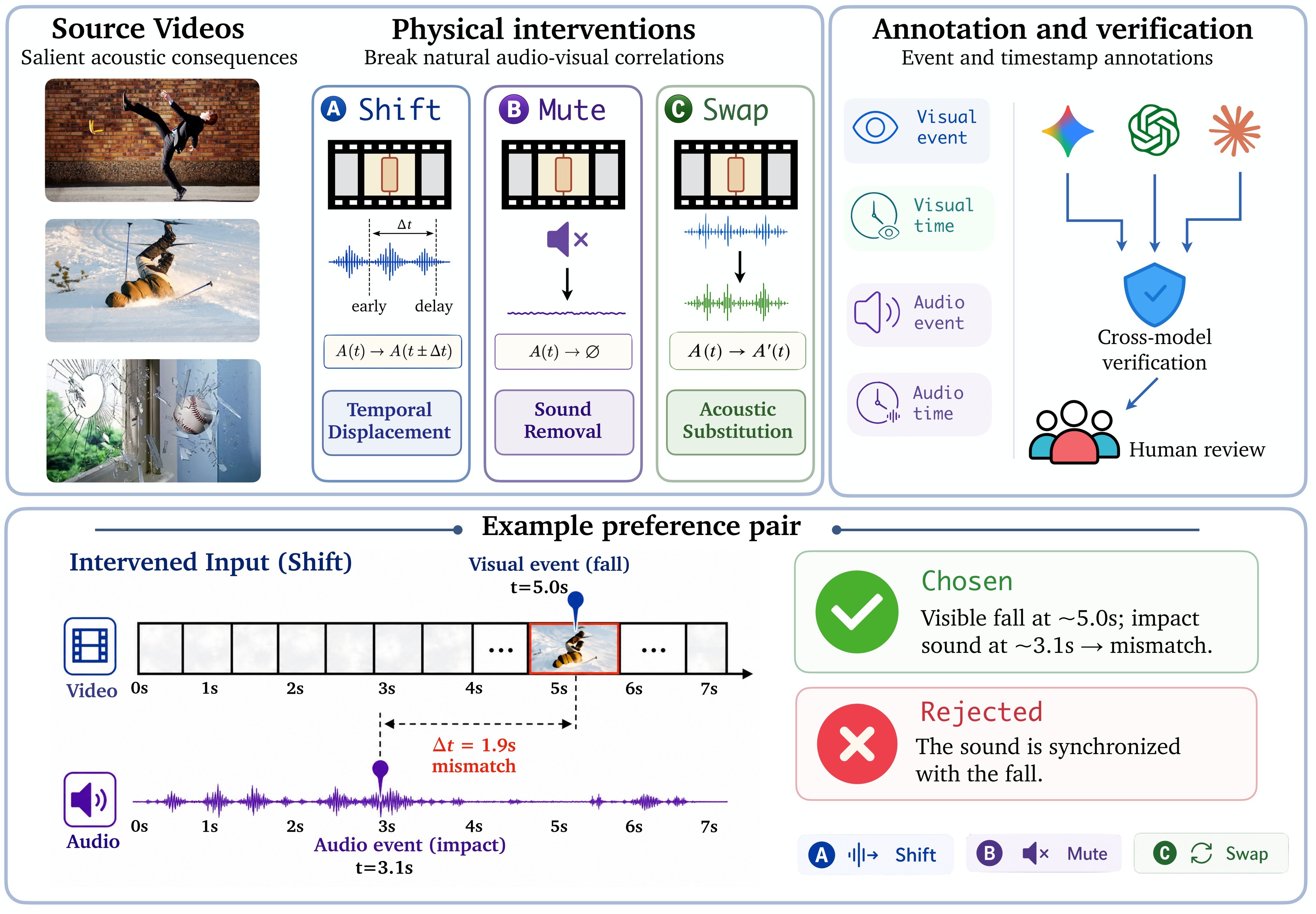
Figure 3. Data construction pipeline for intervention-derived preference pairs. — **Figure 3. Data construction.** Source videos are annotated, cross-verified, filtered, intervened with Shift/Mute/Swap, and converted into chosen/rejected training pairs.

Samples are retained only when visual annotations agree within \(\epsilon_v = 0.8\) seconds or overlapping frame units, audio timestamps are human-verified within \(\epsilon_a = 0.5\) seconds of Gemini's prediction, events are clear and acoustically salient, and the intervention has an unambiguous correct answer. This strict filtering is important because the benchmark would otherwise measure annotation noise rather than audio-visual grounding.

The alignment recipe in Figure 4 uses two stages. Stage 1 performs SFT warm-up on intervention-derived data so the model learns the response pattern of checking audio. Stage 2 applies DPO to intervention preference pairs mixed with general video data, so the model prefers audio-verified responses without over-specializing to synthetic counterfactual prompts.

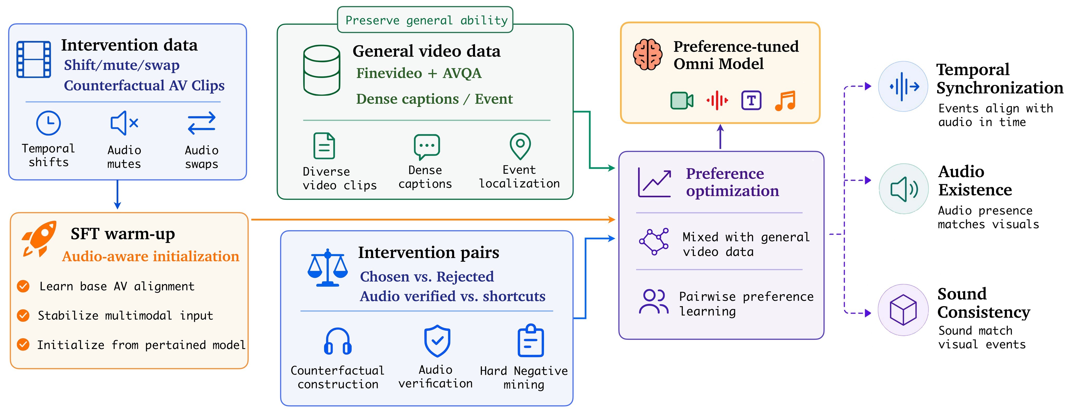
Figure 4. Two-stage intervention-driven alignment pipeline. — **Figure 4. Alignment pipeline.** The paper's alignment study combines targeted intervention preferences with general video preferences to reduce shortcut behavior while preserving broad video understanding.

The preference sources are deliberately separated. Original synchronization preferences teach ordinary alignment; self-sampled negatives correct the model's own post-SFT errors; counterfactual temporal preferences force distinction between original and shifted clips; FineVideo-derived description, localization, attribution, and audio-visual QA preferences regularize the model on general video understanding.

Experiments And Results

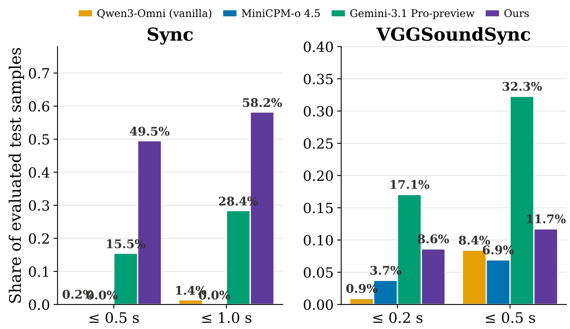
The diagnostic experiments compare API-tested models - Gemini-3.1-Pro, MiMo-V2.5, and Nemotron-3-Nano-Omni - with locally evaluated MiniCPM-o-4.5, Qwen3-Omni, and Ming-Omni-2.0. GPT-5.5 is discussed qualitatively but omitted from the main accuracy table because the tested interface did not support direct audio input for video. The controlled training experiments use Qwen3-Omni-30B as the trainable backbone, evaluate general capability on Video-MME, LVBench, DailyOmni, and WorldSense, and test out-of-distribution synchronization on VGGSoundSync.

The core diagnostic result is that many models look strong on original videos and fail once the audio-video correlation is broken. The strongest examples in Table 3 are Qwen3-Omni's temporal-sync drop from 100.0 to 1.4 under Shift, MiniCPM-o-4.5's 80.7 average gap, and MiMo-V2.5's 78.4 average gap.

Model	Size	Temporal orig	Shift	Audio-existence orig	Mute	Sound-consistency orig	Swap	Avg gap
Gemini	N/A	54.9	46.5	100.0	13.4	93.6	18.3	56.8
MiniCPM-o-4.5	9B	83.8	13.7	100.0	19.0	95.8	4.9	80.7
Nemotron-3-Omni	30B	35.9	26.8	66.2	4.2	88.7	19.9	46.6
Qwen3-Omni	30B	100.0	1.4	95.1	0.0	75.4	37.3	77.3
Ming-Omni-2.0	100B	54.2	20.1	95.7	54.9	90.1	15.5	49.8
MiMo-V2.5	311B	73.9	9.9	99.3	2.1	89.4	15.3	78.4

Figure 5. Failure-mode heatmap across evaluated models. — **Figure 5. Failure-mode heatmap.** The paper reports that audio hallucination dominates: Mute Hallucination and Swap False-Match are high across models, while symmetric false-silence or false-mismatch errors are much rarer.

Figure 6. Prediction breakdown across Shift, Mute, and Swap interventions. — **Figure 6. Prediction breakdown.** On Mute and Swap, errors mostly collapse to hallucinated synced answers. On Shift, Qwen3-Omni answers synced on 98% of inputs, while several models show partial offset sensitivity but unreliable direction recovery.

The alignment results in Table 4 support the paper's second half: targeted preference optimization can reduce shortcut behavior without a broad alignment tax. The final 10K DPO recipe, described as CTP + FV-D + FV-A-L in the text, improves Sync from 34.3 to 83.1 and VGGSync from 36.8 to 56.4, while raising the six-benchmark average from 51.3 to 63.3.

Recipe	Sync	VGGSync	V-MME	LVB	WS	DO	Avg
Qwen3-Omni-30B	34.3	36.8	69.2	49.1	50.3	68.2	51.3
SFT w/ CTP + FV-D + FV-AL	76.1	46.7	43.8	40.8	48.2	66.9	53.8
DPO w/ SP	75.4	55.7	69.3	50.9	49.8	69.0	61.7
DPO w/ OP + FV-D + LV-MCQA	83.0	56.6	69.2	50.4	49.9	67.6	62.8
DPO w/ CTP + FV-D + FV-A	82.6	55.9	69.1	50.8	49.9	67.3	62.6
Ours	83.1	56.4	70.1	52.1	50.3	67.9	63.3

OP means original-sync preferences, SP means SFT-policy negatives, CTP means counterfactual temporal preferences, FV-* means FineVideo-derived preferences, and LV-MCQA is LLaVA-Video multiple-choice QA.

Figure 7. Difficulty-band robustness on VGGSoundSync offsets. — **Figure 7. Difficulty-band robustness.** The paper argues that synchronized-video accuracy alone is misleading: models must detect nonzero offsets and should show a sensible difficulty curve as \(|\Delta|\) gets smaller.

Figure 8a. Synchronization accuracy across binary, three-way, and direction metrics.

Figure 8b. Offset localization coverage under tolerance thresholds. — **Figure 8. Complementary synchronization results.** The first panel focuses on synced/desynced and direction decisions; the second checks whether predicted offsets land close to the true temporal displacement.

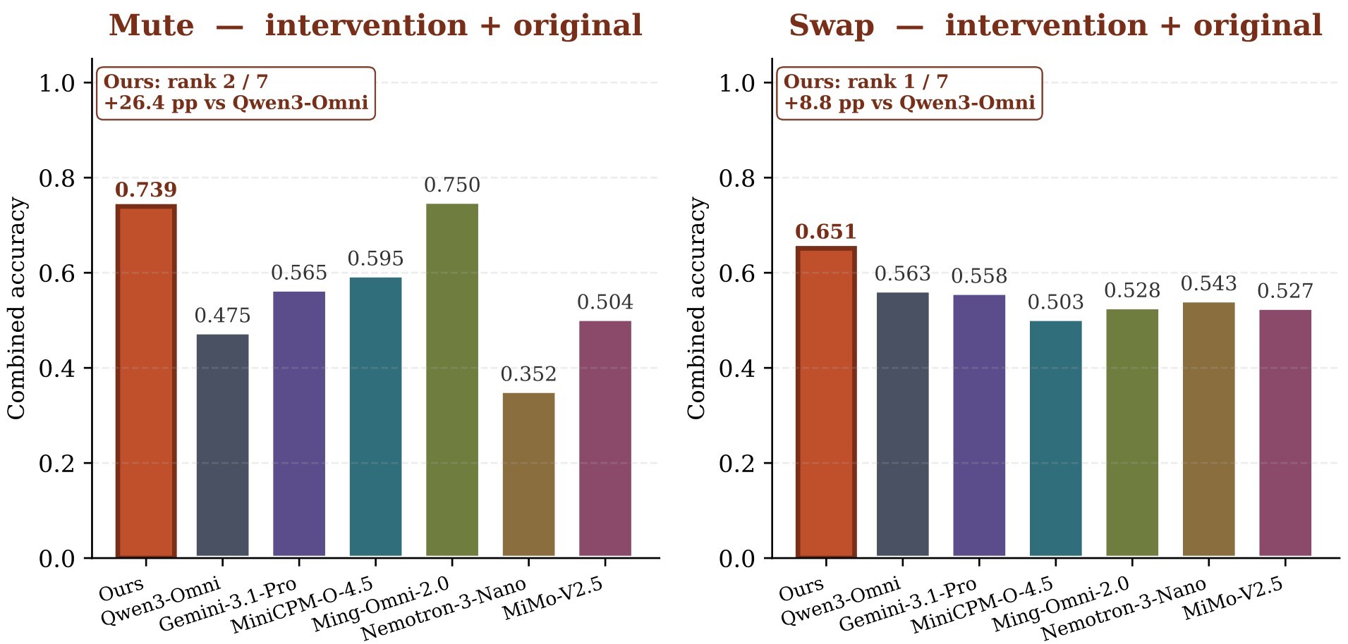
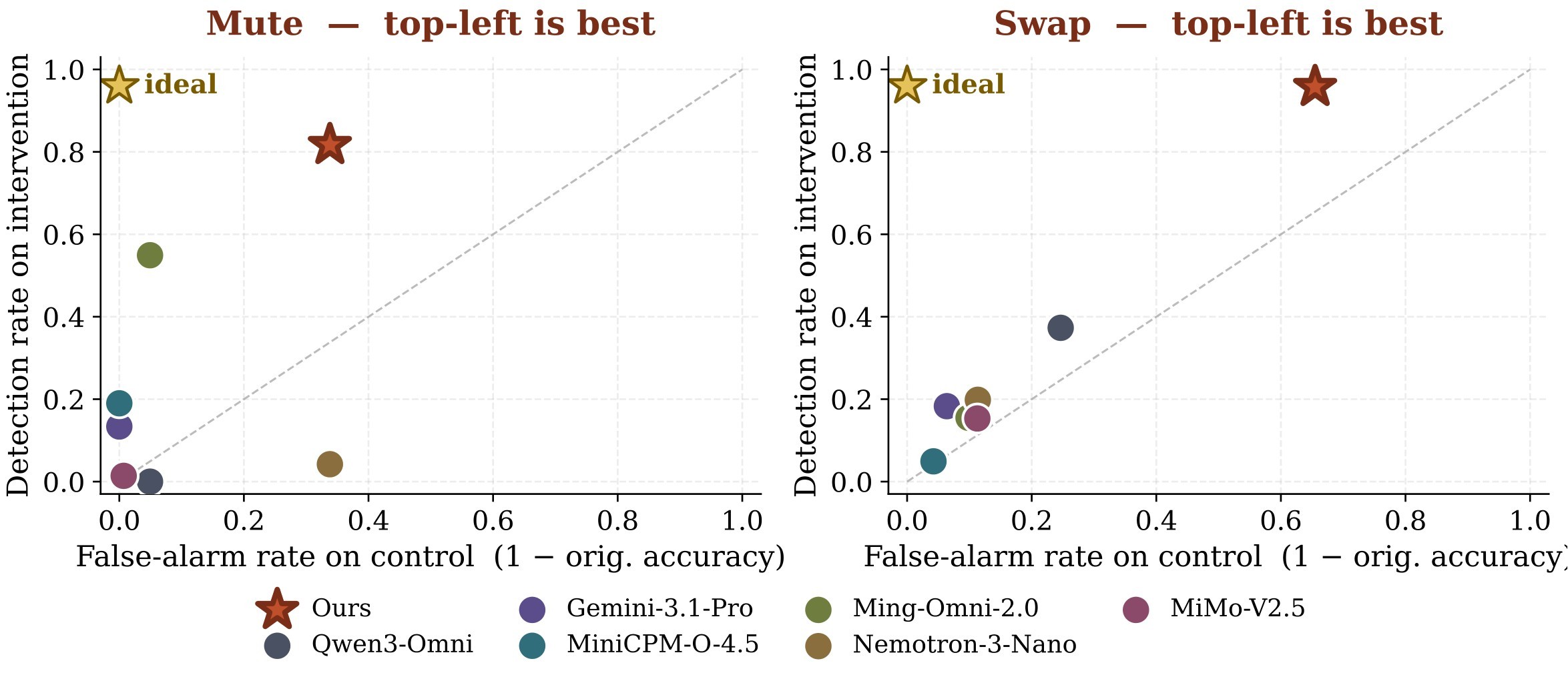
The paper's broader intervention result is more tentative but still useful. Starting from the best temporal recipe, the authors add a small amount of Mute/Swap SFT. The resulting model ranks first on Swap and second on Mute, with a reported 28 percentage-point average gain over vanilla Qwen3-Omni across Shift, Mute, and Swap. Figure 9 and Figure 10 support the claim that this is not just a higher false-alarm setting.

Figure 9. Mute and Swap performance beyond temporal synchronization. — **Figure 9. Beyond temporal synchronization.** The combined Mute/Swap plot supports the claim that intervention-based alignment can extend beyond Shift, though the paper treats this as less complete than the temporal study.

Figure 10. Intervention-control tradeoff between detection and false alarms. — **Figure 10. Intervention-control tradeoff.** The best setting should move toward strong intervention detection with few false alarms on original controls; the paper reports that the trained model moves closer to this region, especially for Swap.

Practical Takeaways

The main limitation is scope. The full training study centers on Qwen3-Omni-30B and primarily validates DPO after SFT for temporal synchronization. The authors explicitly state that the Mute and Swap settings do not yet have a complete training study, and that robustness under broader omni-modal model families, noisy audio, edited videos, and subtle cross-modal inconsistencies remains open.

The most actionable reading is in Table 5.

Reader	Takeaway	Why it matters
Benchmark builder	Include counterfactual audio edits, not only naturally correlated audio-video clips.	Natural correlations let visual priors masquerade as audio grounding.
Model evaluator	Report separate Shift, Mute, Swap, false-alarm, and offset-direction metrics.	A single average can hide synchronized-default behavior and audio hallucination.
Alignment researcher	Prefer targeted preference data plus general-video regularization over plain SFT mixing.	The source results show SFT can improve Sync while degrading broad video benchmarks.
Product or safety reviewer	Treat Thud-style evaluation as a diagnostic stress test, not a deployment guarantee.	Passing intervention tests does not eliminate failures on out-of-distribution sounds or edited videos.

Figure Provenance

All included display figures were copied from the monthly ranking JPEG cache for p017; no source-side rasterization was performed during digest writing. Table 6 maps each digest figure to the extraction-side figure label and original LaTeX asset.

Digest anchor	Source figure id	Source label	Local asset	Original LaTeX asset
Figure 1	`fig_0001`	`fig:motivation`	`figs/fig001_01_motivation_fig_3.jpg`	`Fig/motivation_fig_3.pdf`
Figure 2	`fig_0002`	`fig:pilot_cases`	`figs/fig002_01_fig2_v2.jpg`	`Fig/fig2_v2.pdf`
Figure 3	`fig_0009`	`fig:data-construction`	`figs/fig009_01_DataDPO_splitAv3.jpg`	`Fig/DataDPO_splitAv3.pdf`
Figure 4	`fig_0010`	`fig:preference_optimization`	`figs/fig010_01_DataDPO_splitB_reduced.jpg`	`Fig/DataDPO_splitB_reduced.pdf`
Figure 5	`fig_0003`	`fig:failure_heatmap`	`figs/fig003_01_heatmap_v2.jpg`	`Fig/heatmap_v2.pdf`
Figure 6	`fig_0004`	`fig:breakdown`	`figs/fig004_01_prediction_breakdown_v2.jpg`	`Fig/prediction_breakdown_v2.pdf`
Figure 7	`fig_0005`	`fig:vgg_diff`	`figs/fig005_01_fig3_vgg_difficulty_curve.jpg`	`Fig/fig3_vgg_difficulty_curve.pdf`
Figure 8	`fig_0006`	`fig:headline-accuracy` plus flattened labels `fig:sync-results-combined` and `fig:offset-coverage`	`figs/fig006_01_fig1_headline_accuracy.jpg`; `figs/fig006_02_fig4_offset_coverage.jpg`	`Fig/fig1_headline_accuracy.pdf`; `Fig/fig4_offset_coverage.pdf`
Figure 9	`fig_0007`	`fig:beyond_sync`	`figs/fig007_01_fig1_hero_combined_narrow.jpg`	`Fig/fig1_hero_combined_narrow.pdf`
Figure 10	`fig_0008`	`fig:falsealarm`	`figs/fig008_01_fig3_pareto_det_vs_falsealarm.jpg`	`Fig/fig3_pareto_det_vs_falsealarm.pdf`

Reference coverage: evidence anchors problem framing, Thud framing, interventions, key equations, annotation, alignment method, setup, shortcut results, alignment results, beyond temporal, and limitations are all referenced above. Figure anchors Figure 1, Figure 2, Figure 3, Figure 4, Figure 5, Figure 6, Figure 7, Figure 8, Figure 9, and Figure 10, plus table anchors Table 1, Table 2, Table 3, Table 4, Table 5, and Table 6, are also linked from explanatory text.