Source-first digest for monthly 2026_05 rank 24, rank_id p073.
- Routing status:
pandoc_failed; used flattened TeX plusequations.jsonandfigures.json - PDF extraction: not used
Motivation / Background
SpatialBench asks whether current spatial foundation models are actually all-round 3D players rather than systems that look strong only on their home benchmarks. The source paper motivates the benchmark by pointing to four gaps in prior evaluation: narrow paradigm coverage, inconsistent scene/frame protocols, weak stress testing across input density, and limited coverage of robotics, autonomous driving, egocentric, and wrist-view domains.
The headline scale is large for a 3D geometry benchmark: 19 datasets, 546 scenes, five spatial domains, 41 model variants, six model paradigms, five task suites, and four input density regimes. The main claims and support scores are summarized in Table 1, and the benchmark composition is condensed in Table 2.
The paper is not only a leaderboard. It uses the benchmark to argue that current models split into different operating regimes: full-context feed-forward models define the high-accuracy region when memory is available, bounded-memory models handle long sequences, and domain-matched data matters more than simply adding unrelated training data. The authors then introduce DA-Next-5M and Depth-Anything-Next as a targeted response to the egocentric and wrist-view data gap.
Claims And Evidence
Support scores in Table 1 are source-support scores, not independent reproduction scores. A score of 5 means the claim is directly backed by source text, tables, equations, or figures. A score of 4 means the paper gives strong internal evidence but the claim still depends on benchmark representativeness, hardware assumptions, or unreproduced training details.
| Claim id | Main claim | Support | Evidence anchors |
|---|---|---|---|
| C1 | SpatialBench is a broad, deterministic, cross-paradigm benchmark for spatial foundation models. | 5 | scale, benchmark design, stats table, overview figure |
| C2 | The density protocol is designed to separate single-frame, sparse, medium, and dense failure modes. | 5 | density protocol, key equations, main results |
| C3 | Full-context models are the accuracy upper bound under bounded input length, but they hit memory limits on long dense sequences. | 4 | memory and accuracy evidence, operating snapshot, memory scaling, main results |
| C4 | Data quality and domain alignment matter more than raw dataset count, especially for egocentric and wrist-view scenes. | 4 | data quality evidence, data/performance figure, OOD figure, domain coverage |
| C5 | DA-Next-5M and Depth-Anything-Next directly target the embodied-domain gap and report large gains over DA3-Giant on sparse and medium inputs. | 4 | DA-Next data, DA-Next architecture, DA-Next samples, main results |
| C6 | Test-time training is not a universal free lunch: it helps most on dense long sequences and is inconsistent on sparse or medium inputs. | 5 | TTT evidence, TTT table |
| C7 | GT depth priors strongly improve depth, but camera priors are not always obeyed by prior-aware models. | 4 | prior evidence, prior table, bad-case figure |
| C8 | The benchmark has explicit limitations around evaluation cost, H200-specific memory assumptions, hyperparameter tuning, and incomplete model coverage. | 5 | limitations |
Core Technical Idea
The core idea is to evaluate spatial foundation models under a controlled factorial protocol rather than a single average score. SpatialBench fixes the evaluated scene/frame indices, normalizes each dataset into RGB, metric depth, camera-to-world pose, and intrinsics, and then evaluates the same models across domain, viewpoint, dynamics, source type, input density, and task type. Figure 1 is the source paper's benchmark overview.
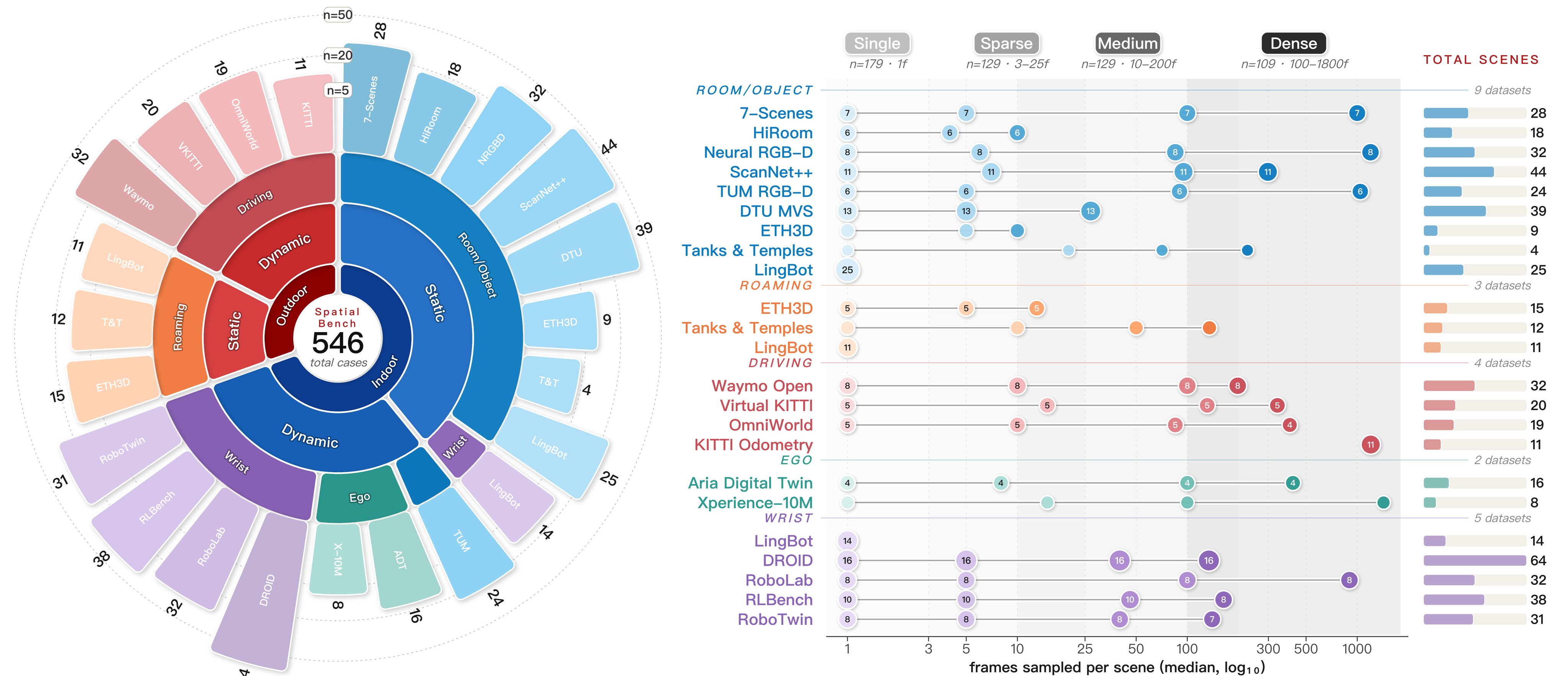
| Benchmark axis | Source value | Digest interpretation |
|---|---|---|
| Source datasets | 19 | Covers indoor, outdoor, driving, egocentric, and wrist-view data. |
| Evaluation scenes | 546 | Same scene can be evaluated under multiple density regimes. |
| Evaluation frames | 72,540 | Appendix total across the benchmark composition table. |
| Model variants | 41 | Six paradigms: optimization, feed-forward, online/streaming, chunk-wise, SLAM, and TTT. |
| Task suites | 5 | Camera pose, camera trajectory, depth, dense reconstruction, and prior-enhanced prediction. |
| Density regimes | 4 | Single, sparse, medium, dense. |
Table 2. SpatialBench coverage. This table condenses the source abstract, introduction, and appendix benchmark-composition table.
The multi-density protocol is the part that makes the benchmark more diagnostic than a pooled leaderboard. Single-frame evaluation isolates monocular depth priors. Sparse selection stresses wide-baseline reconstruction from only a few frames. Medium keeps more overlap while still limiting the budget. Dense preserves long-horizon temporal continuity while capping cost. The equations in Table 3 capture the selection and metric objects that matter most.
| Object | Source equation | Why it matters | ||||
|---|---|---|---|---|---|---|
| Sparse set cover | \(\mathcal{S}=\arg\max_{S\subseteq\mathcal{F}, | S | \le K} | \bigcup_{f\in S} V_f | \) | Sparse frames are chosen for voxel coverage, not arbitrary temporal spacing. |
| Medium budgeted set cover | \(\mathcal{S}=\arg\max_{S\subseteq\mathcal{F}, F_{\min}(N)\le | S | \le F_{\max}(N)} | \bigcup_{f\in S} V_f | \) | Medium inputs preserve overlap while adapting the number of frames to sequence length. |
| Dense stride | \(s=\lceil N/T\rceil\), with \(T=500\) | Dense evaluation keeps temporal continuity but avoids unbounded evaluation cost. | ||||
| Rotation accuracy | \(\mathrm{RAcc}_{x}= | \mathcal{P} | ^{-1}\sum_{(i,j)\in\mathcal{P}}\mathbf{1}[e^R_{ij}\lt x]\) | Pairwise camera rotation is thresholded over all ordered view pairs. | ||
| Pose AUC | \(\mathrm{AUC}_{x_{\max}}=x_{\max}^{-1}\int_0^{x_{\max}}\mathrm{Acc}_x\,dx\) | AUC@30 is the main compact camera-pose score in the result tables. | ||||
| Depth AbsRel | \(\mathrm{AbsRel}= | \Omega_D | ^{-1}\sum_{p\in\Omega_D} | D_p-\hat{D}_p | /D_p\) | Lower AbsRel is the main depth-error column used in headline comparisons. |
| DA-Next objective | \(\mathcal{L}=\mathcal{L}_{depth}+\alpha\mathcal{L}_{grad}+\mathcal{L}_{ray}+\mathcal{L}_{pmap}+\mathcal{L}_{scale}\) | DA-Next trains depth, gradients, rays, point maps, and metric scale jointly. | ||||
| DA-Next scale target | \(S= | \Omega | ^{-1}\sum_{p\in\Omega}\|\mathbf{P}_p\|_2\) | Absolute metric scale is supervised separately while dense predictions are normalized. |
Table 3. Key equations. The equations come from the flattened TeX and equations.json; HTML-sensitive comparison signs are written with \lt.
Method Details
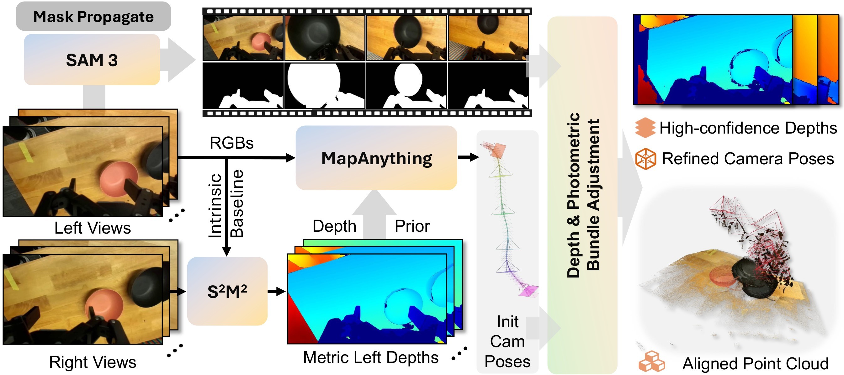
SpatialBench normalizes heterogeneous datasets into a shared per-scene representation and fixed JSON scene records. The paper gives special attention to the DROID wrist-view subset because it is a key embodied-domain gap: stereo depth is estimated with S2M2, initial poses come from MapAnything, dynamic gripper/contact regions are masked with SAM3, and depth/photometric bundle adjustment refines camera poses and globally aligned point clouds. The pipeline is shown in Figure 2.
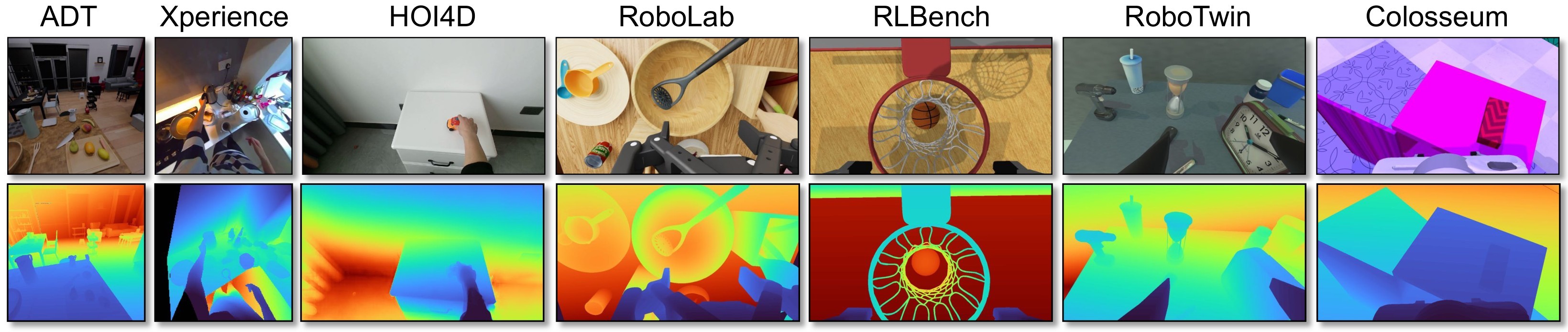
DA-Next-5M is the paper's data-side response to the benchmark's largest gap. The source appendix describes 22K sequences and 5.5M frames from egocentric and robot wrist-view sources, with image sequences, depth maps, intrinsics, and camera extrinsics. Figure 3 shows the visual variety, and Table 4 condenses the dataset statistics.
| Component | View | Real/synthetic | Frames | Scenes |
|---|---|---|---|---|
| Xperience | Ego | Real | 400K | 100 |
| Aria Digital Twin | Ego | Synthetic | 86K | 232 |
| Colosseum | Wrist | Synthetic | 334K | 1,837 |
| HOI4D | Ego | Real | 739K | 2,466 |
| RLBench | Wrist | Synthetic | 1.2M | 5,120 |
| Robolab | Wrist | Synthetic | 158K | 132 |
| RoboTwin | Wrist | Synthetic | 2.6M | 11,923 |
Table 4. DA-Next-5M composition. The values are taken from the appendix dataset-statistics table.
Depth-Anything-Next builds on DA3-Giant but adds explicit metric-scale prediction and optional camera conditioning. It takes image frames and, when available, camera intrinsics/poses; patch tokens, camera tokens, and scale tokens are jointly processed by a transformer encoder; Dual-DPT heads produce depth and ray maps; and an MLP regresses the scalar metric scale. The model architecture is shown in Figure 4.
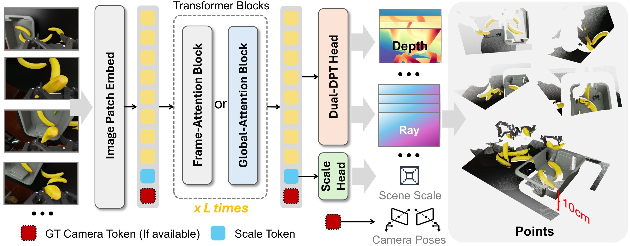
The training objective combines five terms: depth, depth gradients, ray maps, point maps, and scale. The source appendix also explains a scale-normalization step: world points, depths, and translations are normalized by a per-scene scale \(S\), while \(S\) itself becomes the regression target of the scale head. Stochastic pose conditioning injects ground-truth camera information into some batches and uses learnable camera tokens otherwise. This makes the model usable both with and without camera priors at inference.
Experiments And Results
The main result table compares 41 variants across all density regimes. Table 5 condenses the rows and columns most relevant to the paper's claims.
| Model / family | Sparse AbsRel | Sparse AUC@30 | Medium AbsRel | Medium AUC@30 | Dense status / note | Digest interpretation |
|---|---|---|---|---|---|---|
| VGGT | 0.105 | 0.700 | 0.125 | 0.687 | OOM | Strong bounded-input baseline, but full-context memory does not scale. |
| \(\pi^3\) | 0.092 | 0.742 | 0.082 | 0.749 | Runs dense, but ATE 16.39 | Strong sparse/medium pose, weaker long-horizon trajectory. |
| DA3-Giant | 0.095 | 0.785 | 0.086 | 0.776 | OOM | High full-context accuracy, especially reconstruction F-score, but no dense run. |
| DA-Next | 0.050 | 0.809 | 0.035 | 0.819 | OOM | Large depth and pose gains over DA3-Giant on sparse/medium inputs. |
| LingBotMap-S | 0.138 | 0.650 | 0.114 | 0.647 | Dense AUC@30 0.627, ATE 3.470 | Online model with strong dense scalability. |
| DA3-Streaming | 0.095 | 0.785 | 0.091 | 0.767 | Dense F-score 0.516 | Chunk/streaming variant with best reported dense F-score in the main table. |
| Scal3R | 0.114 | 0.732 | 0.147 | 0.670 | Dense ATE 2.396 | TTT method with strong dense trajectory behavior. |
| LoGeR* | 0.077 | 0.708 | 0.083 | 0.714 | Dense AUC@30 0.598, ATE 4.598 | TTT improves dense scale but can regress sparse/medium AUC versus base \(\pi^3\). |
Table 5. Main result digest. The source table contains additional metrics, including trajectory, point-cloud, timing, parameter counts, and average columns.
The paper's key architectural finding is the accuracy/scalability tradeoff. At \(N=800\), full-context feed-forward methods occupy the best depth-accuracy region, as shown in Figure 5. But the memory curve in Figure 6 explains why dense long-horizon evaluation flips the deployment question: full-context models can run out of memory, while streaming, chunk-wise, and TTT variants keep processing by limiting active context.
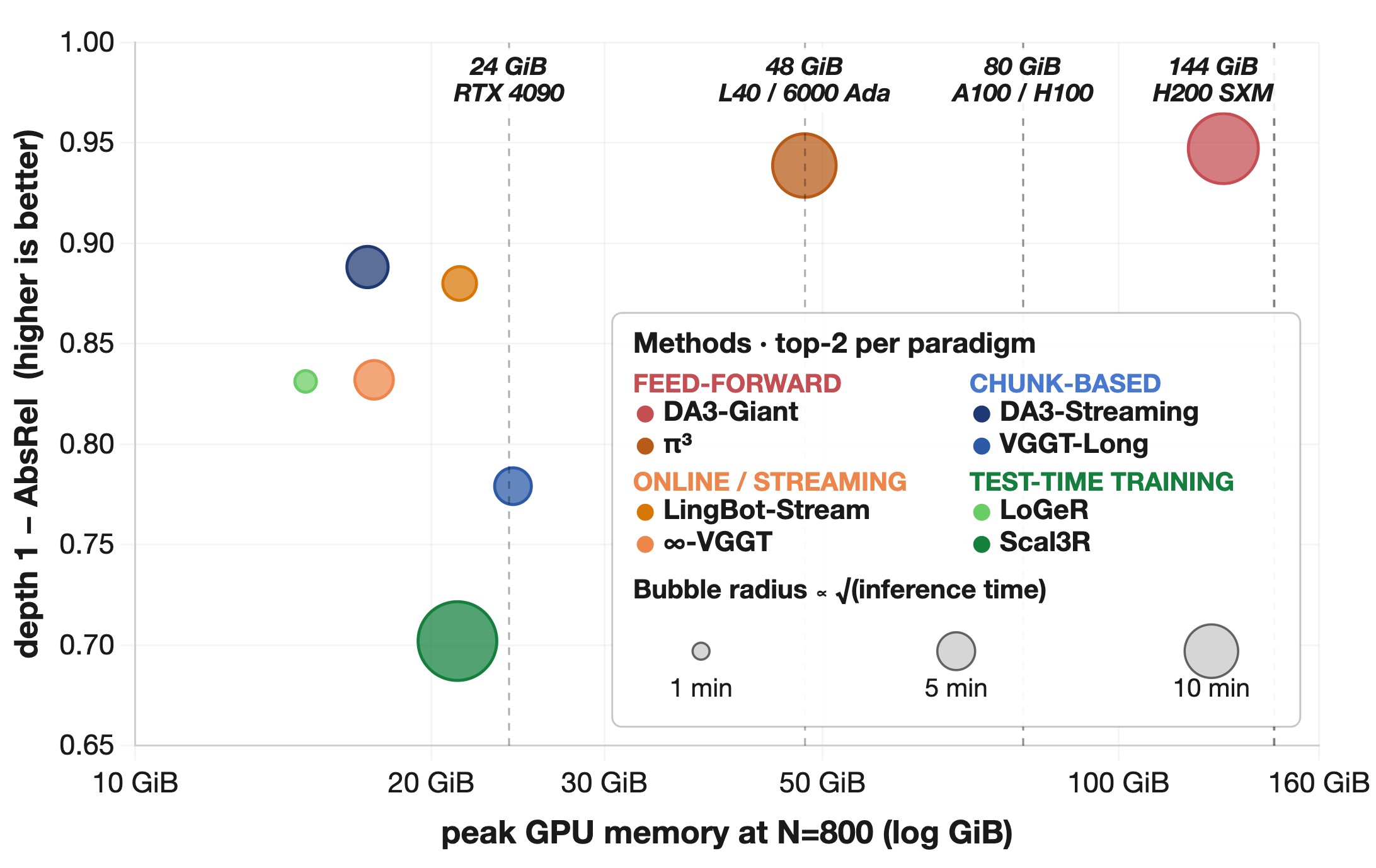
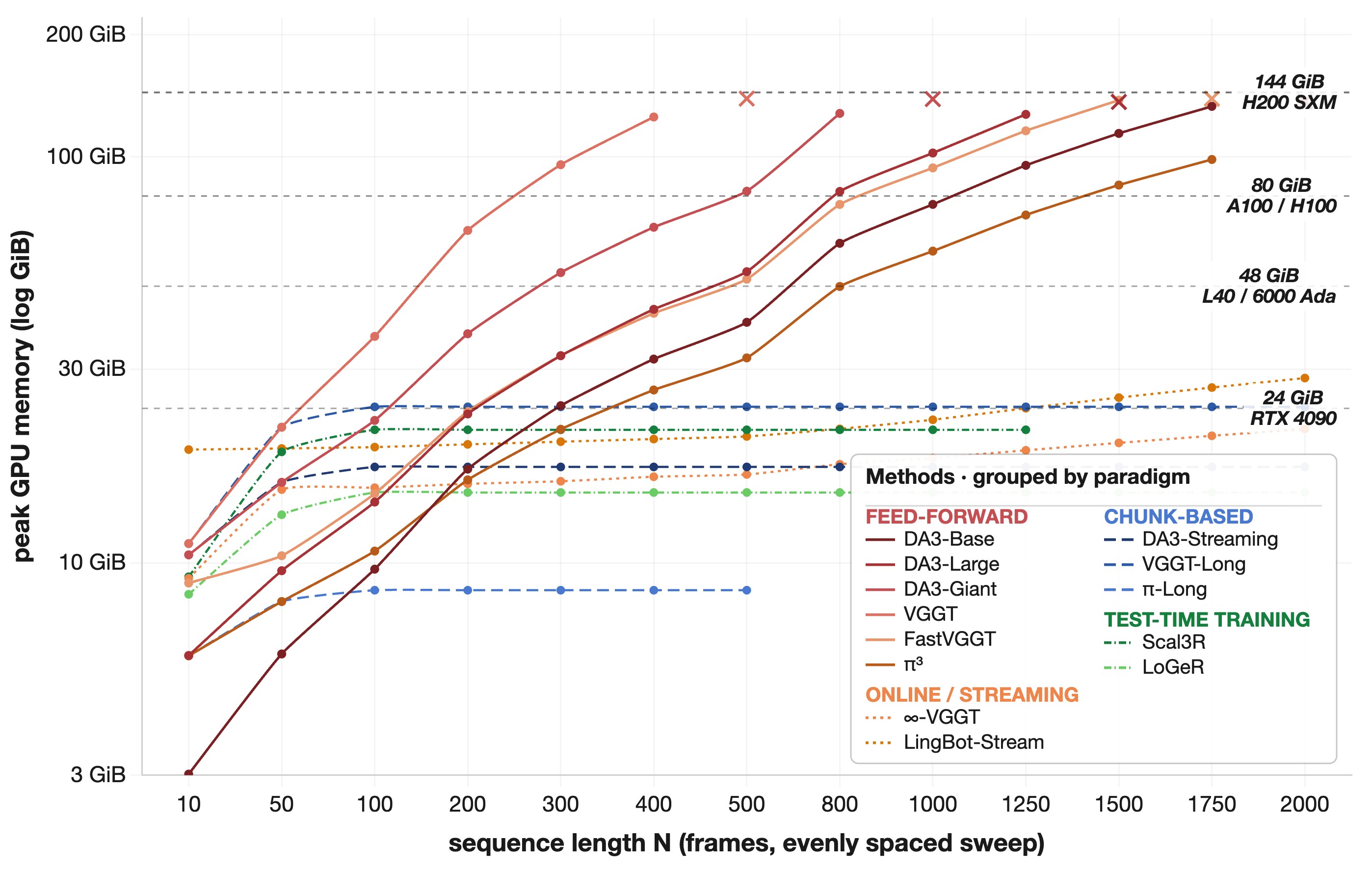
The data analysis supports a second claim: more data helps, but domain and annotation quality are decisive. Figure 7 shows training coverage versus benchmark performance, while Figure 8 shows that egocentric and wrist-view scenes are the most severe OOD regions. The paper uses this to justify DA-Next-5M rather than just enlarging the generic training mixture.
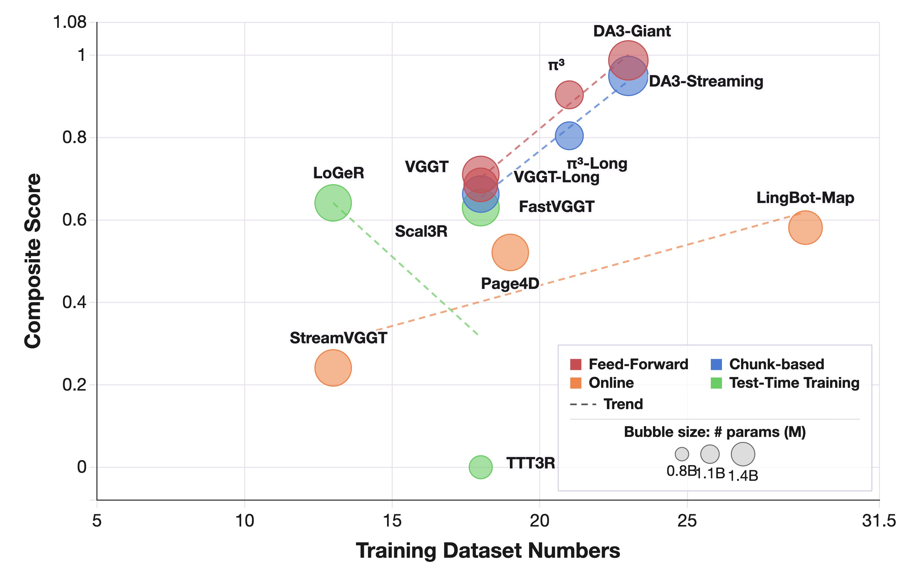
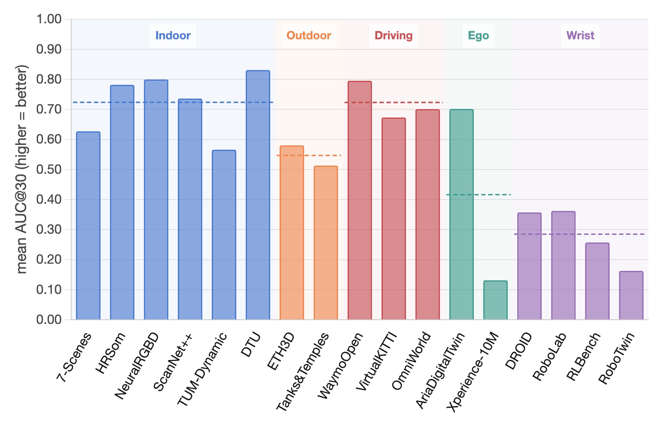
The test-time training result is nuanced. Table 6 shows that TTT helps most in dense long sequences, where base models either degrade or cannot run, but it can be neutral or harmful on sparse/medium inputs.
| Regime | Pair | AUC@30 change | ATE change | Digest interpretation |
|---|---|---|---|---|
| Sparse | CUT3R to TTT3R | 0.519 to 0.470 | n/a | TTT hurts pairwise pose in short, discontinuous inputs. |
| Sparse | VGGT to Scal3R | 0.700 to 0.732 | n/a | One sparse exception where TTT improves AUC. |
| Sparse | \(\pi^3\) to LoGeR | 0.742 to 0.708 | n/a | TTT hurts sparse AUC. |
| Medium | CUT3R to TTT3R | 0.469 to 0.493 | 2.68 to 2.34 | TTT helps both metrics for this pair. |
| Medium | VGGT to Scal3R | 0.687 to 0.670 | 0.73 to 0.40 | Better trajectory, worse pairwise AUC. |
| Medium | \(\pi^3\) to LoGeR | 0.749 to 0.714 | 0.57 to 0.57 | Worse AUC, flat trajectory. |
| Dense | CUT3R to TTT3R | 0.165 to 0.321 | 25.5 to 21.1 | Dense sequence length is where TTT clearly helps. |
| Dense | VGGT to Scal3R | OOM to 0.480 | OOM to 2.40 | Scal3R runs where VGGT OOMs. |
| Dense | \(\pi^3\) to LoGeR | 0.524 to 0.598 | 16.4 to 4.60 | Strong dense trajectory gain. |
Table 6. TTT versus base models. The source wraptable reports these values as base-to-TTT arrows.
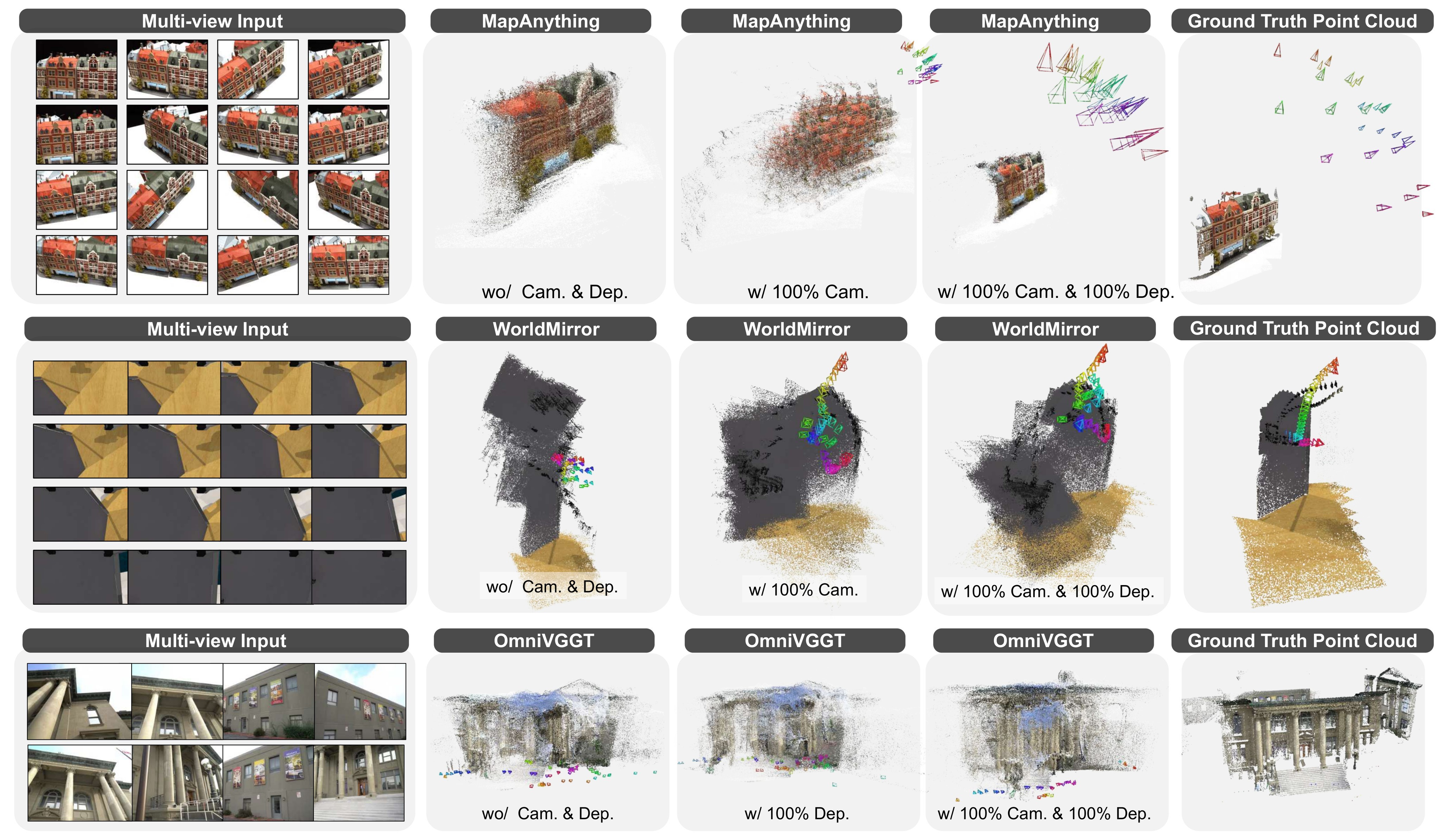
Prior-aware models do not become perfect when given GT information. Table 7 summarizes the sparse/medium prior ablation. Depth priors consistently drive depth metrics close to ground truth. Camera priors are more mixed: DA3-Giant and MapAnything strongly adhere to GT poses, but OmniVGGT, \(\pi^3\)-X, and WorldMirror sometimes partially override the camera prior, especially in challenging scenes.
| Finding | Representative source values | Digest interpretation |
|---|---|---|
| Depth priors strongly reduce depth error | Sparse MapAnything AbsRel 0.153 to 0.029 with depth prior; sparse \(\pi^3\)-X 0.084 to 0.009 with depth prior | Depth can become near-GT when depth itself is supplied as an auxiliary input. |
| Camera priors strongly help some models | Sparse DA3-Giant AUC@30 0.785 to 0.984 with camera prior; medium DA3-Giant AUC@30 0.776 to 0.987 | Some architectures use camera priors almost as intended. |
| Camera priors are not universally obeyed | Medium WorldMirror AUC@30 0.674 to 0.838 with camera prior, not near perfect; qualitative failures remain | The paper argues that some models override or underuse injected camera poses. |
| Both priors do not eliminate all errors | Medium OmniVGGT with both priors: AUC@30 0.910, ATE 0.639, F-score 0.693 | Even with both prior types, nontrivial camera/trajectory/reconstruction errors remain. |
Table 7. Prior ablation digest. The full source table reports depth, camera, trajectory, and point-cloud metrics for sparse and medium regimes.
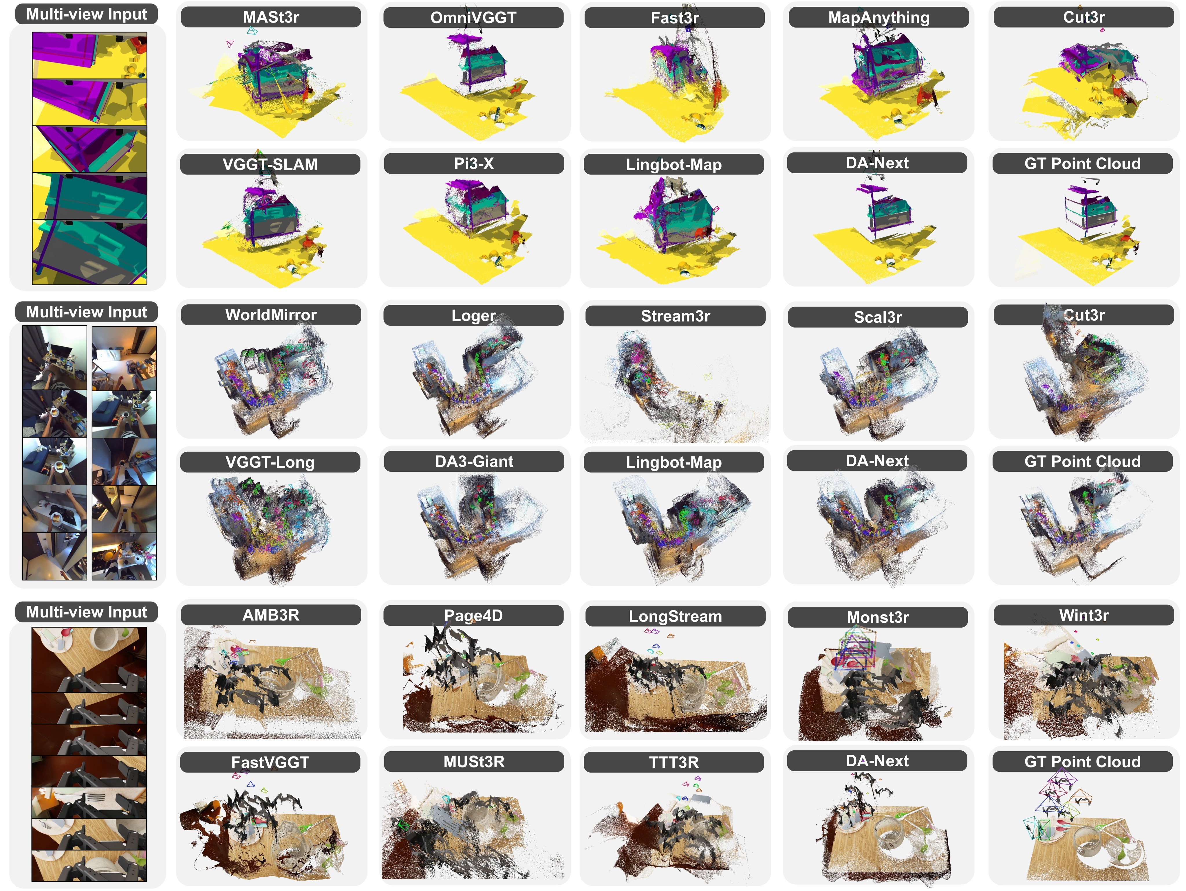
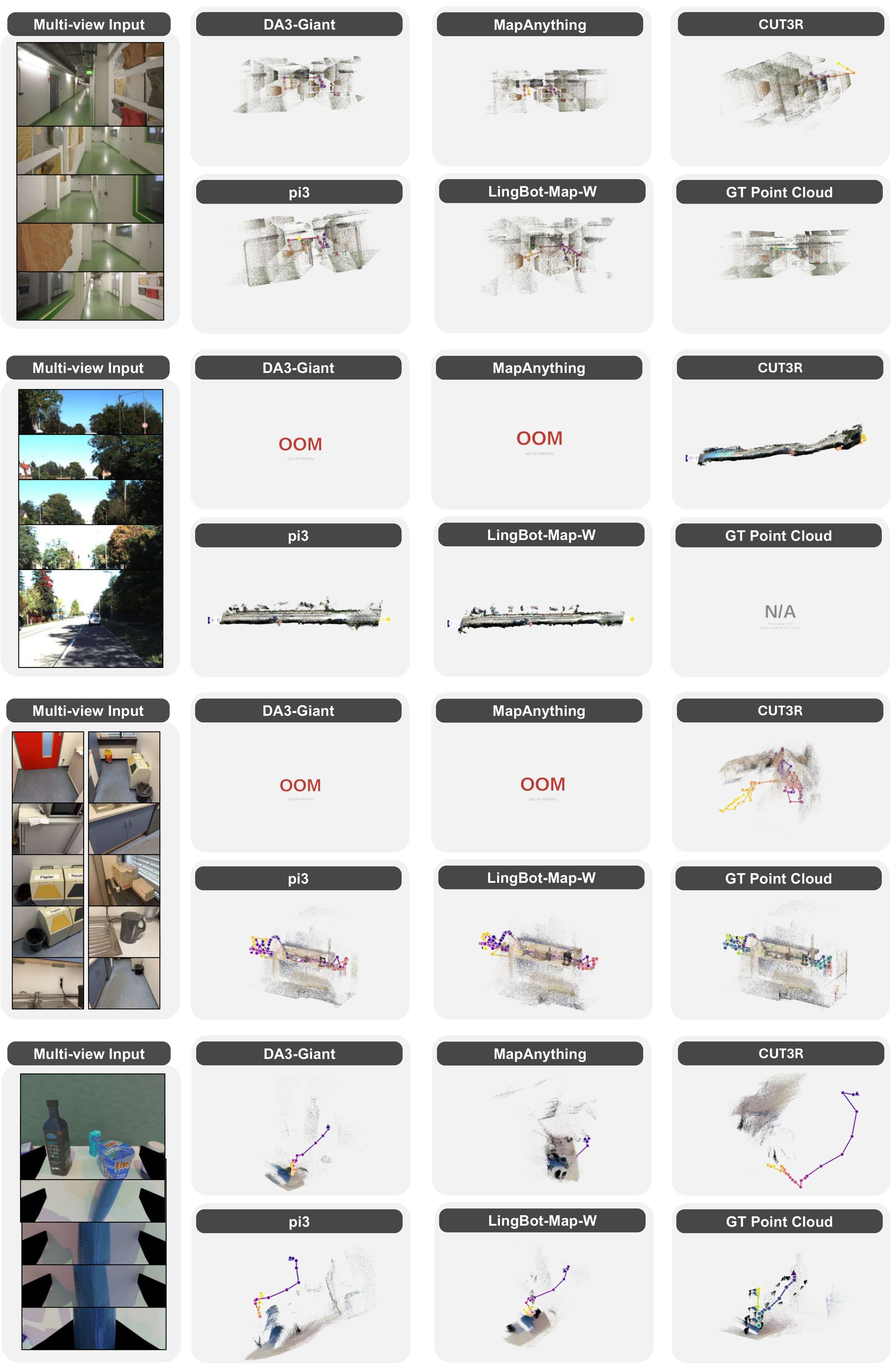
The qualitative figures support the same story visually. Figure 9 compares representative multi-view reconstructions and reports that DA-Next gives sharper geometry and more accurate trajectory under challenging viewpoints. Figure 10 broadens this to four benchmark cases, including dense outdoor driving and wrist-view OOD input. Figure 11 shows the prior-enhanced failure modes mentioned above.
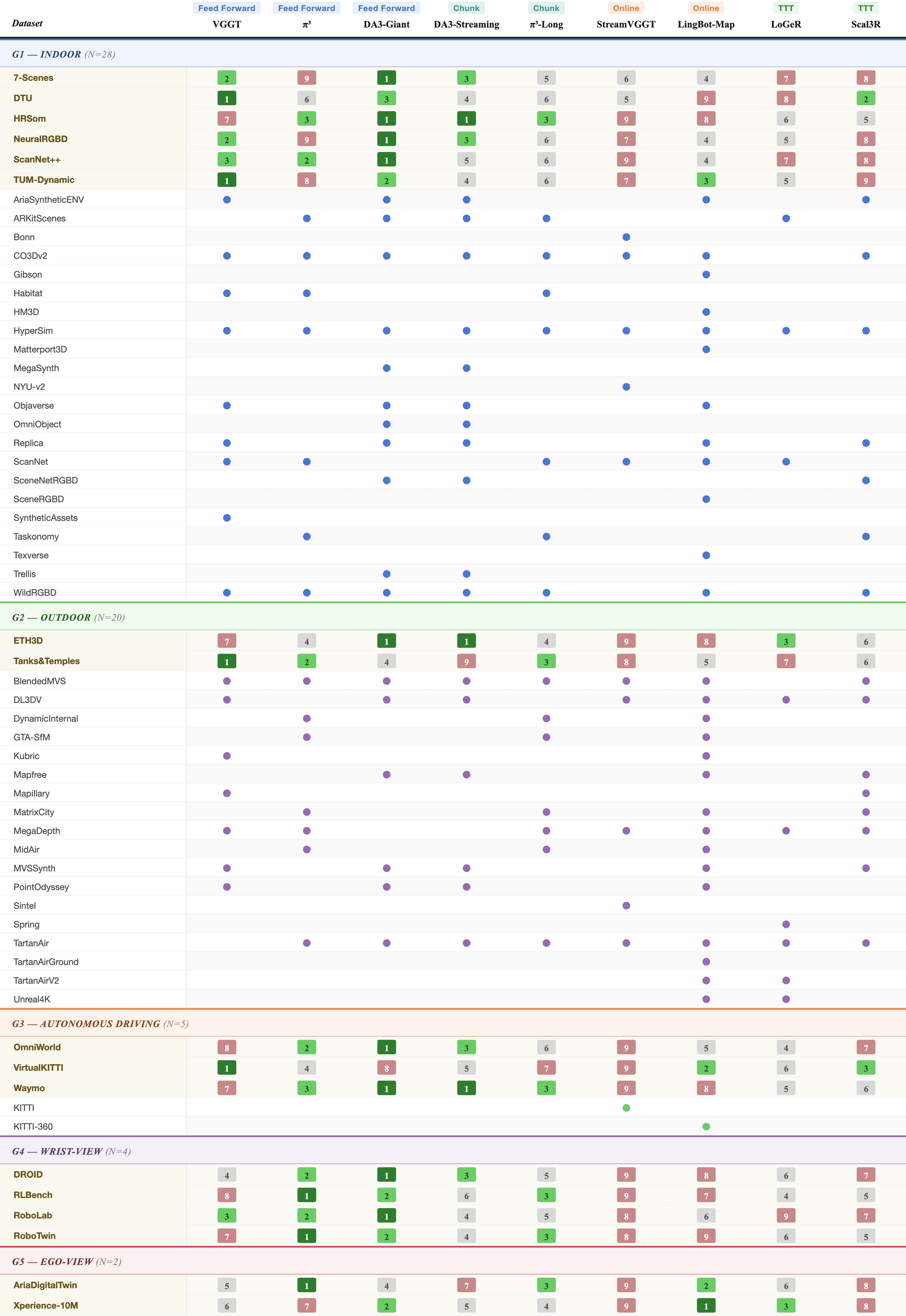
The appendix also gives a deployment-oriented view: Figure 12 ranks representative methods by domain group and overlays whether training data covers that domain. Its practical message is direct: average benchmark rank is not enough when the target deployment domain differs from the training mixture.
Practical Takeaways
1. Use SpatialBench as a diagnostic benchmark, not only as a leaderboard. The important question is which density, domain, and task suite matches the downstream system. 2. For bounded multi-view inputs, full-context feed-forward models are still the accuracy reference point. For dense long sequences or memory-constrained deployment, bounded-memory, chunk-wise, online, or TTT models become necessary. 3. Data curation should prioritize target-domain coverage and annotation quality. The paper's strongest empirical argument is that egocentric and wrist-view failures remain even for otherwise strong spatial foundation models, and DA-Next improves by adding targeted embodied data. 4. If a method accepts priors, do not assume GT priors make evaluation trivial. The prior ablation shows depth and camera priors behave differently, and some models still fail qualitatively under hard cases. 5. The benchmark numbers are hardware- and configuration-sensitive. The limitations in the source discussion explicitly note H200 memory assumptions, evaluation cost, limited hyperparameter tuning, and incomplete coverage of newly released methods.
The source limitations are concrete: evaluating 41 models over dense regimes is expensive; all evaluations use H200 GPUs with 141 GB VRAM, so larger-memory hardware could change behavior; task- or scene-specific hyperparameter tuning is outside scope; and the authors cannot cover all newly released models at submission time.
Reference Coverage
Anchor coverage links: claims, scale, benchmark design, overview figure, benchmark stats, density protocol, key equations, data curation, DROID pipeline, DA-Next data, DA-Next samples, DA-Next data table, DA-Next architecture evidence, DA-Next architecture figure, main results evidence, main results table, memory evidence, operating snapshot, memory scaling, data quality evidence, data/performance figure, domain OOD figure, TTT evidence, TTT table, prior evidence, prior table, qualitative evidence, main visualization, representative cases, bad cases, domain coverage, limitations.