EarlyTom: Early Token Compression Completes Fast Video Understanding

Source-first digest for checked paper rank 8, rank_id p008.

Routing status: success
PDF extraction: not used

Motivation / Background

Video LLMs often become slow before generation even starts: each video frame contributes many visual tokens, and the system has to encode those frames, process visual tokens, and prefill the language model before the first output token appears. EarlyTom's central observation is that many previous token-compression methods prune after the vision encoder or inside the LLM, so they leave a large part of time-to-first-token (TTFT) untouched.

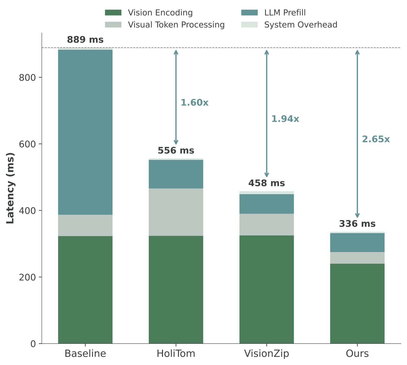
The paper profiles this bottleneck directly. In the baseline LLaVA-OneVision-7B setup, vision encoding is 323 ms and 36.3% of TTFT; for HoliTom and VisionZip, once LLM prefill is compressed, vision encoding rises to 55.8% and 68.4% of TTFT. This makes Figure 3 the motivation figure: faster Video-LLM serving needs compression earlier than the LLM prefill boundary.

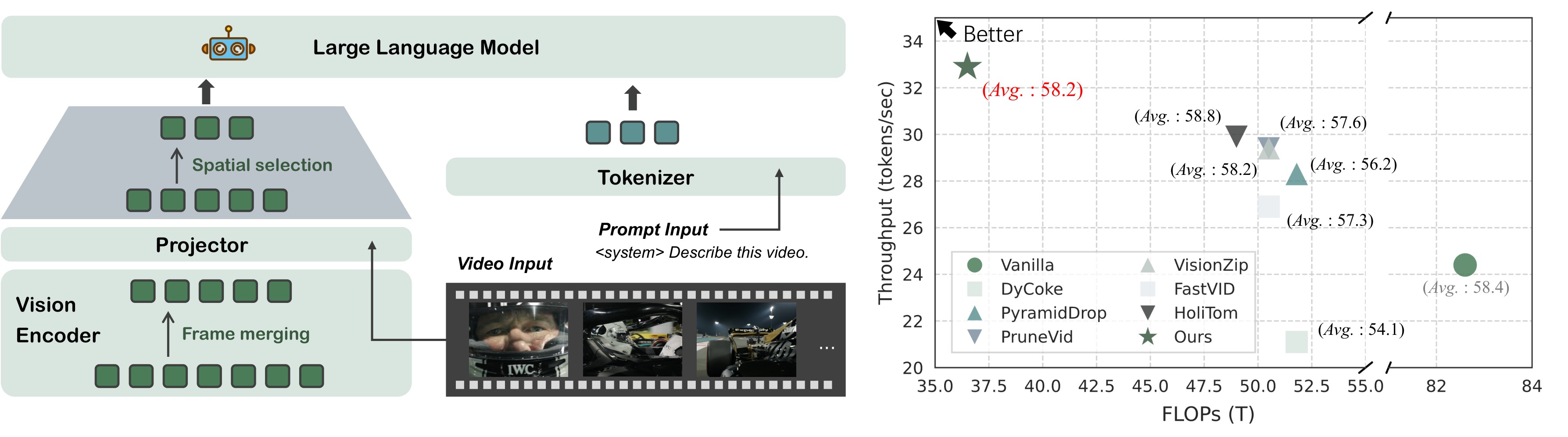
EarlyTom is a training-free inference method. It moves part of compression into the vision encoder with streaming frame merging, then performs a decoupled spatial token selection step before LLM decoding. The teaser in Figure 1 frames the target use case as practical video understanding acceleration, and Figure 4 shows the two-stage pipeline.

**Figure 1. EarlyTom teaser and efficiency/accuracy trade-off.** The original caption says the paper targets faster video understanding by compressing tokens at the early vision-encoder stage and shows EarlyTom on a FLOPs-throughput-performance scatter plot. I place it here because it summarizes the practical deployment motivation.

**Figure 2. Video sink tokens.** The original caption visualizes videos across datasets and shows that certain frame/region tokens attract disproportionately high attention. This motivates why naive top-K attention selection can over-select structural sink tokens and miss semantic information from other frames.

**Figure 3. TTFT latency composition.** The source caption decomposes TTFT into vision encoding, visual token processing, LLM prefill, and system overhead. It reports a 2.65x TTFT reduction over the baseline at 10% token retention on an NVIDIA A100 GPU.

Claims And Evidence

Claim id	Main claim	Support	Evidence anchors
C1	Vision encoding is a first-order TTFT bottleneck for video LLM inference, especially after late-stage token compression reduces LLM prefill.	5	TTFT profile, 7B main results, 7B TTFT breakdown
C2	Compressing earlier inside the vision encoder gives materially lower TTFT and FLOPs than late-stage training-free compression while preserving near-baseline benchmark accuracy.	5	teaser, pipeline, frame equations, 7B main results, 0.5B results
C3	The two modules, inner-encoder frame merging and decoupled spatial selection, are complementary.	4	module ablation, layer ablation, frame distribution, sampling ablation
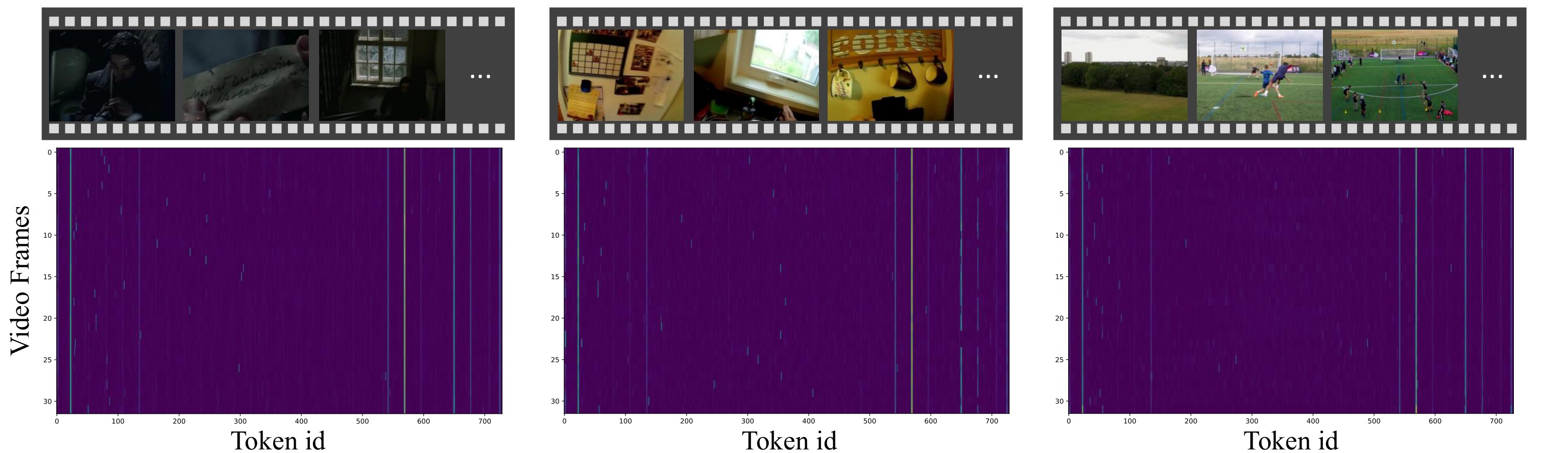
C4	Decoupled spatial selection is motivated by attention sink behavior and provides a better speed/accuracy balance than global top-K or random sampling.	4	attention sink, supplementary sink visualizations, sampling ablation
C5	EarlyTom generalizes beyond one exact LLaVA-OneVision-7B configuration to a smaller LLaVA-OneVision model and other backbones.	4	0.5B results, 0.5B TTFT breakdown, LLaVA-Video results, Qwen2.5-VL results
C6	The method is immediately practical as a training-free system intervention, but the evidence is bounded to the tested Video-LLM stacks and prefill/TTFT metrics.	3	implementation settings, future work

Scores are support-from-paper scores, not independent reproduction scores. Efficiency claims are strong for the reported GPUs, models, and benchmarks. General deployment claims are capped because the paper evaluates selected Video-LLM families and does not optimize decoding-stage generation.

Core Technical Idea

EarlyTom treats Video-LLM latency as a system problem: if visual tokens are only reduced after the vision encoder, the encoder still pays for the full video. The method therefore compresses temporal redundancy during selected vision-encoder layers, then compresses spatial tokens before feeding the LLM.

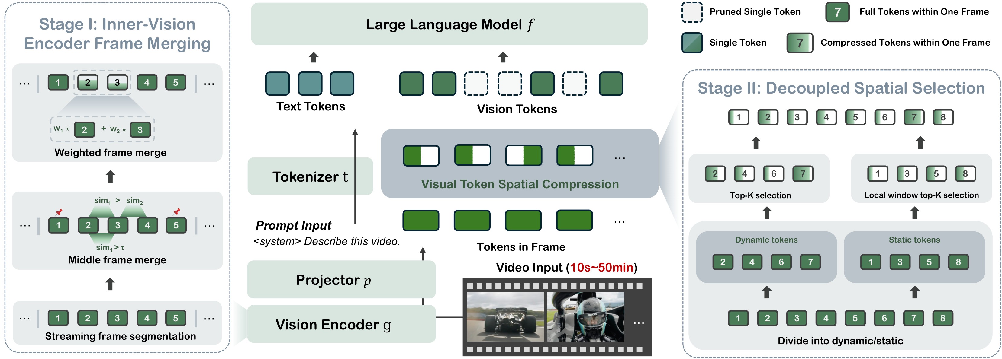
Figure 4. Overall pipeline of EarlyTom. — **Figure 4. Overall pipeline.** The source caption describes two stages: inner-vision encoder frame merging for temporal compression, followed by decoupled spatial token selection over dynamic and static frame features. This is the paper's main method figure.

The two-stage structure in Figure 4 is:

Stage I, inner-vision encoder frame merging. Segment the video by streaming frame similarity, preserve segment endpoints, and merge redundant middle frames inside selected vision-encoder layers.
Stage II, decoupled spatial token selection. Split merged frame features into dynamic and static groups. Dynamic frames use global top-K attention selection; static frames use local-window top-K selection so sink tokens do not dominate all retained positions.
System co-design. Static token selection is partly offloaded to CPU while GPU handles dynamic selection, using otherwise idle CPU capacity to reduce processing overhead.

The key design point is not a new trained model. It is a training-free placement and selection strategy: remove temporal redundancy before the full vision stack has processed every frame, then reduce spatial tokens without relying blindly on global attention magnitudes.

Method Details

Bottleneck And Sink Analysis

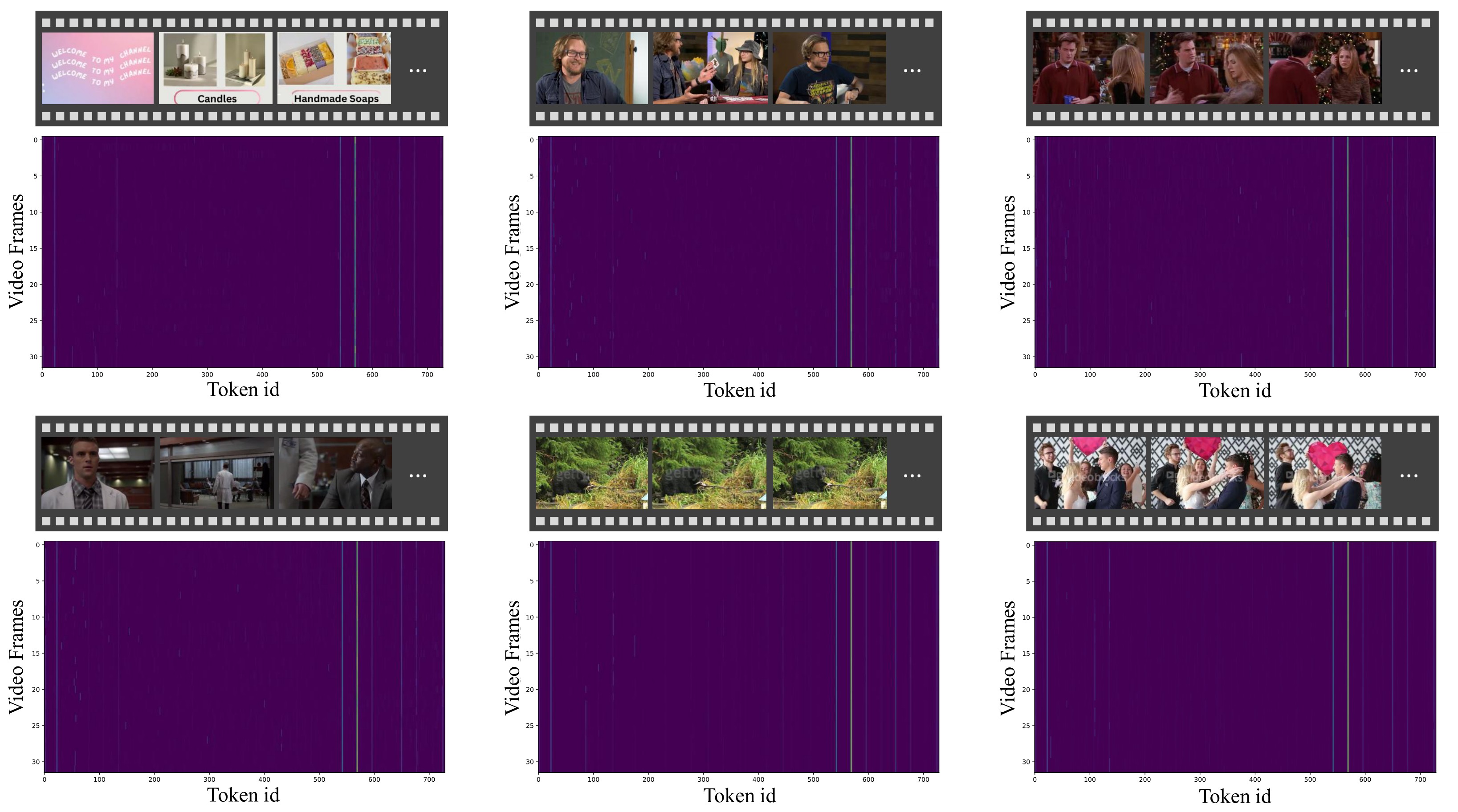
EarlyTom starts from two empirical observations. First, Figure 3 shows that vision encoding is a large part of TTFT. Second, Figure 2 shows that attention maps contain sink-like spatial tokens that attract high attention across frames. The source text formalizes the sink issue with attention

\mathrm{A}(i,j)=\frac{Q_i K_j^\top}{\sqrt{d}},

and states that sink tokens satisfy

\lVert Q_{\mathrm{sink}}\rVert_2 \gg \lVert Q_p\rVert_2,

so attention can be dominated by structural attractors rather than content-bearing regions. This is the reason the paper does not simply apply global top-K attention selection everywhere.

Inner Vision Encoder Frame Compression

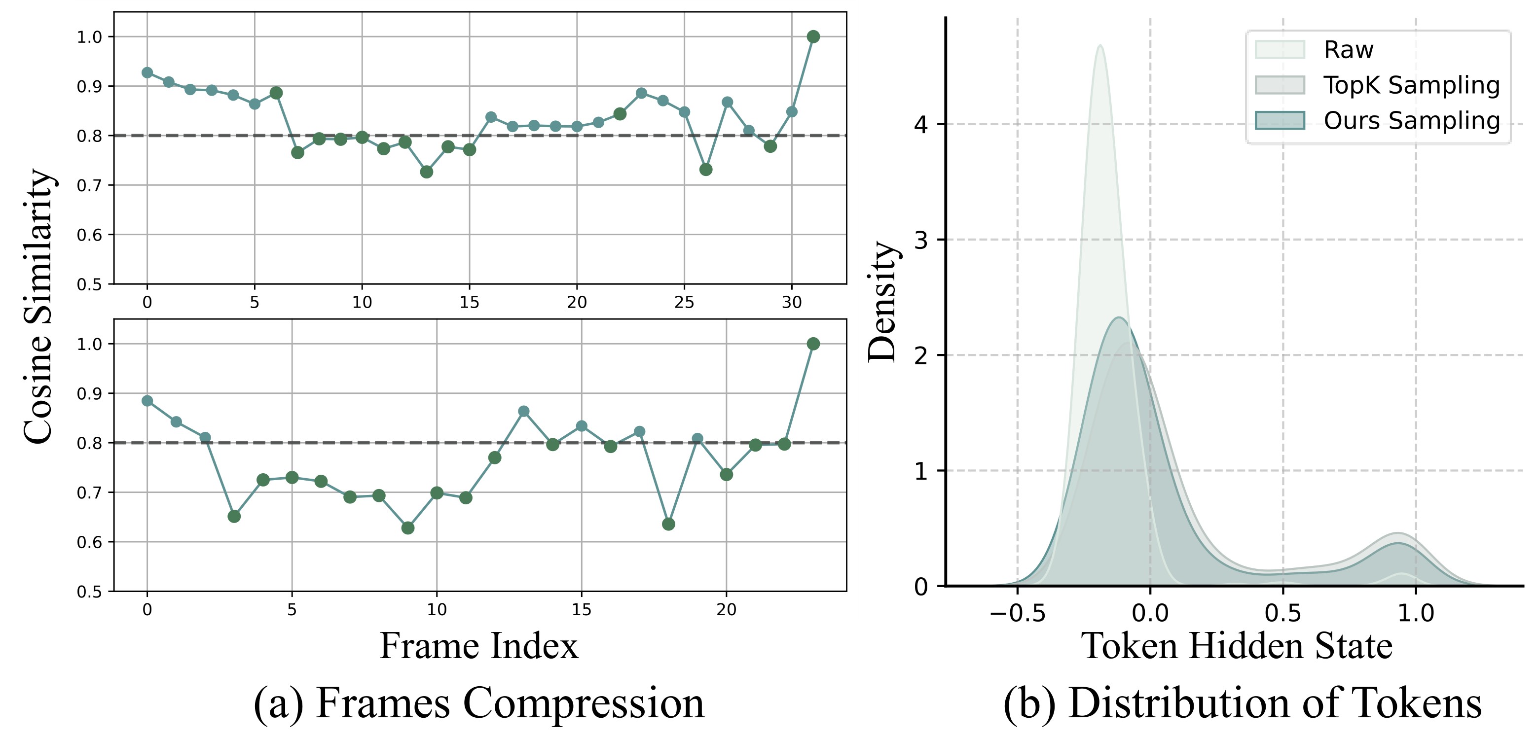
**Figure 5. Frame compression and token distribution.** The source caption shows cosine similarity changes across frame indices at selected vision-encoder layers and compares raw-token, top-K, and EarlyTom token distributions. This figure supports the layer-selection and distribution-preservation logic.

The frame-compression module in Figure 5 first computes frame-to-frame similarity by averaging cosine similarity at corresponding spatial positions. It smooths similarity with an exponential moving average:

\begin{aligned} \hat{s}_t &= \alpha s_t + (1 - \alpha)\hat{s}_{t-1}, \\ \text{break if } \hat{s}_t &\lt \tau_{\mathrm{seg}}. \end{aligned}

Middle frames are candidates for merging, while segment head and tail frames are preserved. A pair is merged only when it is similar enough and is a local similarity maximum:

\begin{aligned} \mathrm{merge}(F_i,F_{i+1}) \quad \mathrm{iff} \quad \begin{cases} s_i>\tau_{\mathrm{merge}} \\ s_i>s_{i+1}. \end{cases} \end{aligned}

The merged feature is a similarity-weighted average:

\hat{F}=\frac{s_iF_i+s_{i+1}F_{i+1}}{s_i+s_{i+1}}.

The paper's intent is conservative: merge only redundant middle frames, keep temporal boundaries, and use similarity weights to avoid a crude average that blurs uneven temporal variation.

Decoupled Spatial Token Selection

After frame merging, EarlyTom divides features into dynamic and static frame sets:

\hat{F}^d \in \mathbb{R}^{T \times L \times D}, \qquad \hat{F}^s \in \mathbb{R}^{(N-T) \times L \times D}.

Dynamic frames are the head and tail frames within each segment. They receive global top-K selection because they are expected to contain motion-sensitive changes:

\begin{aligned} \hat{\hat{F}}^d_i &= \hat{F}^d_i[I_i, :], \\ I_i &= \mathrm{TopK}(A_i, \hat{r}), \\ i &\in [1,T]. \end{aligned}

The selection ratio is rescaled after frame compression:

\hat{r} = \frac{r}{\left(\frac{B-N}{B}\right)L}.

Static frames use local-window top-K so retained positions do not collapse onto the same sink tokens:

\begin{aligned} \{W_1,W_2,\dots,W_m\}, \quad M = \left\lceil \frac{L}{w} \right\rceil, \quad w = \left\lfloor \frac{L}{\hat{r}} \right\rfloor. \end{aligned}

Finally, selected dynamic and static tokens are gathered back in original order:

\hat{\hat{F}} = \mathrm{Gather}(\hat{\hat{F}}^d,\hat{\hat{F}}^s).

The implementation settings in Table 8 show that EarlyTom uses inner-LLM merging, EMA factor 0.9, and task-specific segmentation thresholds and merge layers across retained ratios. The experiments use LLaVA-OneVision-0.5B/7B with 32 uniformly sampled frames, SigLIP vision encoding, NVIDIA A100 and RTX 4090 GPUs, NVIDIA Nsight Systems for TTFT, and LMMs-Eval for benchmark evaluation.

Model	Retained ratio	Inner LLM merge	EMA factor	Example segmentation/layers
LLaVA-OneVision-7B	25%	yes	0.9	MVBench: tau_seg 0.8, layers [6,14,20]
LLaVA-OneVision-7B	10%	yes	0.9	MVBench: tau_seg 0.65, layers [8,14,20]
LLaVA-OneVision-0.5B	25%	yes	0.9	MVBench: tau_seg 0.8, layers [8,21,23]
LLaVA-OneVision-0.5B	10%	yes	0.9	MVBench: tau_seg 0.65, layers [8,21,23]

Table 8. Details of the hyperparameters on LLaVA-OneVision. The full source table lists per-benchmark thresholds and merge layers for 25%, 20%, 15%, and 10% retained ratios on both 7B and 0.5B. I include a compact version because it is implementation provenance rather than primary evidence.

Experiments And Results

Main LLaVA-OneVision-7B Results

Table 1 is the main evidence for the headline speed claim. It compares LLaVA-OneVision-7B against training-free compression baselines across MVBench, EgoSchema, LongVideoBench, and VideoMME.

Method	Retained before LLM	FLOPs T lower	FLOPs ratio lower	TTFT ms lower	Throughput higher	Avg score higher	Avg %
LLaVA-OV-7B full	100%	82.6	100.0%	889.9	24.4	58.4	100.0
HoliTom	25%	49.0	59.3%	661.3	29.9	58.8	100.7
EarlyTom	25%	36.5	44.2%	426.3	32.9	58.2	99.7
HoliTom	20%	47.5	57.5%	622.3	30.0	58.8	100.7
EarlyTom	20%	35.1	42.4%	415.3	33.4	58.1	99.3
HoliTom	15%	46.0	55.7%	572.7	27.5	58.2	99.7
EarlyTom	15%	33.6	40.7%	390.6	30.4	57.3	98.1
VisionZip	10%	45.2	54.7%	458.5	28.5	53.5	91.6
HoliTom	10%	44.6	54.0%	556.6	29.0	57.9	99.1
EarlyTom	10%	32.2	39.0%	336.2	31.6	56.2	96.2

Table 1. Performance and accuracy comparison with SoTA methods across benchmarks. This is a compact version of the source table preserving the full baseline, EarlyTom rows, and the strongest recurring comparator rows. The key result is that EarlyTom has the lowest TTFT and FLOPs at every retained ratio shown, while the average score stays within 96.2-99.7% of the full-token baseline.

The strongest headline is the 10% row: EarlyTom reaches 336.2 ms TTFT versus 889.9 ms for the full baseline and 556.6 ms for HoliTom, while keeping average accuracy at 56.2, or 96.2% of the full-token baseline. This directly supports C2, though it also shows the accuracy trade-off under very aggressive compression.

Smaller LLaVA-OneVision Backbone

Table 2 checks whether the method still helps on a smaller LLaVA-OneVision-0.5B model, where there is less LLM-prefill compute to save.

Method	Retained before LLM	FLOPs T lower	FLOPs ratio lower	TTFT ms lower	Throughput higher	Avg score higher	Avg %
LLaVA-OV-0.5B full	100%	45.3	100.0%	413.7	42.7	40.5	100.0
HoliTom	25%	42.3	93.4%	519.4	35.2	41.0	101.2
EarlyTom	25%	29.9	66.0%	331.5	47.8	40.7	100.4
HoliTom	20%	42.2	93.2%	499.4	38.3	40.8	100.7
EarlyTom	20%	29.8	65.8%	313.1	40.6	40.3	99.5
HoliTom	15%	42.1	92.9%	473.9	34.1	40.7	100.4
EarlyTom	15%	29.7	65.6%	311.1	35.1	39.8	98.3
HoliTom	10%	42.0	92.7%	457.1	39.6	40.0	98.8
EarlyTom	10%	29.6	65.3%	280.1	43.9	39.4	97.3

Table 2. Cross-backbone comparison on LLaVA-OneVision-0.5B. The original caption emphasizes performance and accuracy across backbones. The notable result is that EarlyTom remains faster even when HoliTom can become slower than the full 0.5B baseline because its processing overhead offsets prefill savings.

Module And Sampling Ablations

Table 3 isolates the two compression modules.

Method	Retained ratio	MVBench	VideoMME	EgoSchema	Avg
Vanilla	100%	58.3	58.6	60.4	59.1
Only stage 1	73.9%	57.9	57.0	60.3	58.4
Only stage 2	20%	57.3	57.6	60.4	58.4
EarlyTom	20%	57.8	58.1	60.6	58.8

Table 3. Ablation study on the compression module. Stage 1 alone keeps more tokens but still reaches 58.4 average; stage 2 alone also reaches 58.4 at 20% retained ratio; the full method reaches 58.8, supporting the claim that the modules are complementary.

Table 4 explains why the paper uses a middle starting layer rather than always merging as early as possible.

Initial merge layer	TTFT lower	Throughput higher	MVBench	VideoMME	EgoSchema	Avg
Layer 4	380.0	31.6	57.4	57.9	60.4	58.6
Layer 6	387.1	32.3	57.8	58.1	60.4	58.9
Layer 8	421.1	30.7	57.5	58.0	60.4	58.6
Layer 10	436.9	31.1	57.4	58.0	60.6	58.7

Table 4. Frame merging effectiveness across initial compression layers. Layer 4 is fastest, but layer 6 gives the best average accuracy and throughput in the reported 0.2 compression-ratio setting.

Table 5 tests the local-window spatial sampling choice against simpler selection policies.

Sampling	Throughput higher	MVBench	VideoMME	EgoSchema	Avg
Random	35.3	57.0	56.6	59.8	57.8
Top-K	31.5	57.5	57.3	60.4	58.4
EarlyTom	33.4	57.8	58.1	60.6	58.8

Table 5. Ablation study of token sampling ways. Random sampling is fastest but weaker; global top-K is more accurate but slower; EarlyTom's local-window strategy has the best average score with less throughput loss than global top-K.

The supplementary attention maps in Figure 6 make the attention-sink premise less dependent on a single qualitative example.

Figure 6. Supplementary attention sink visualizations. — **Figure 6. Additional attention score distributions.** The source caption shows attention heatmaps from six random videos and says the vertical stripes confirm that attention sinks are common in the vision encoder. I include it because it backs the sampling design rather than only the motivation.

Generalization Across Backbones

Table 6 moves from LLaVA-OneVision to LLaVA-Video-7B.

Model	Method	Retained before LLM	FLOPs T lower	FLOPs ratio lower	TTFT ms lower	Throughput higher	Avg score	Avg %
LLaVA-Video-7B	Vanilla	100%	246.2	100.0%	6429.3	8.1	60.2	100.0
LLaVA-Video-7B	FastV	100%	158.2	64.3%	3494.3	10.0	55.6	92.4
LLaVA-Video-7B	PyramidDrop	100%	159.4	64.7%	3494.8	10.1	56.7	94.2
LLaVA-Video-7B	VisionZip	15%	159.4	64.7%	3241.4	14.2	56.7	94.2
LLaVA-Video-7B	HoliTom	15%	156.6	63.6%	1669.5	17.1	57.7	95.8
LLaVA-Video-7B	EarlyTom	15%	86.4	35.1%	947.4	16.7	56.4	93.7

Table 6. Efficiency comparison with SoTA methods on LLaVA-Video-7B. At 15% retention, EarlyTom cuts TTFT from 6429.3 ms to 947.4 ms and reduces the FLOPs ratio to 35.1%. It is slightly behind HoliTom on throughput and average score, so the support is strongest for latency/FLOPs rather than absolute accuracy.

Table 7 checks a Qwen2.5-VL-7B setting with a maximum of 768 frames and a 23k-token context length.

Method	FLOPs T lower	FLOPs ratio lower	TTFT ms lower	MVBench	VideoMME short	VideoMME medium	VideoMME long	VideoMME avg	Avg score
Qwen2.5-VL-7B full	554.7	100.0%	6842	67.1	76.0	66.0	55.1	65.7	66.4
Average Pooling	91.9	16.6%	4609	56.8	66.4	57.3	51.1	58.3	57.6
Uniform Subsampling	91.9	16.6%	4578	57.7	68.6	59.6	55.0	60.8	59.3
EarlyTom w/o decoupled spatial selection	67.7	12.2%	3667	60.7	71.0	61.6	53.6	62.0	61.4
EarlyTom w/o weighted frame merging	67.7	12.2%	3667	60.7	70.5	62.3	52.7	61.8	61.3
EarlyTom	67.7	12.2%	3667	62.5	70.7	61.6	53.6	61.9	62.2

Table 7. Qwen2.5-VL trivial baselines and ablations. EarlyTom is far faster than the full Qwen2.5-VL-7B setup and outperforms average pooling and uniform subsampling on average score while using fewer FLOPs. The two ablations show that both spatial selection and weighted merging matter, though the gains over ablated EarlyTom are modest.

TTFT Breakdown Figures

Figure 7 expands the 7B TTFT story across retained ratios.

7B retained ratio	Local figure
10%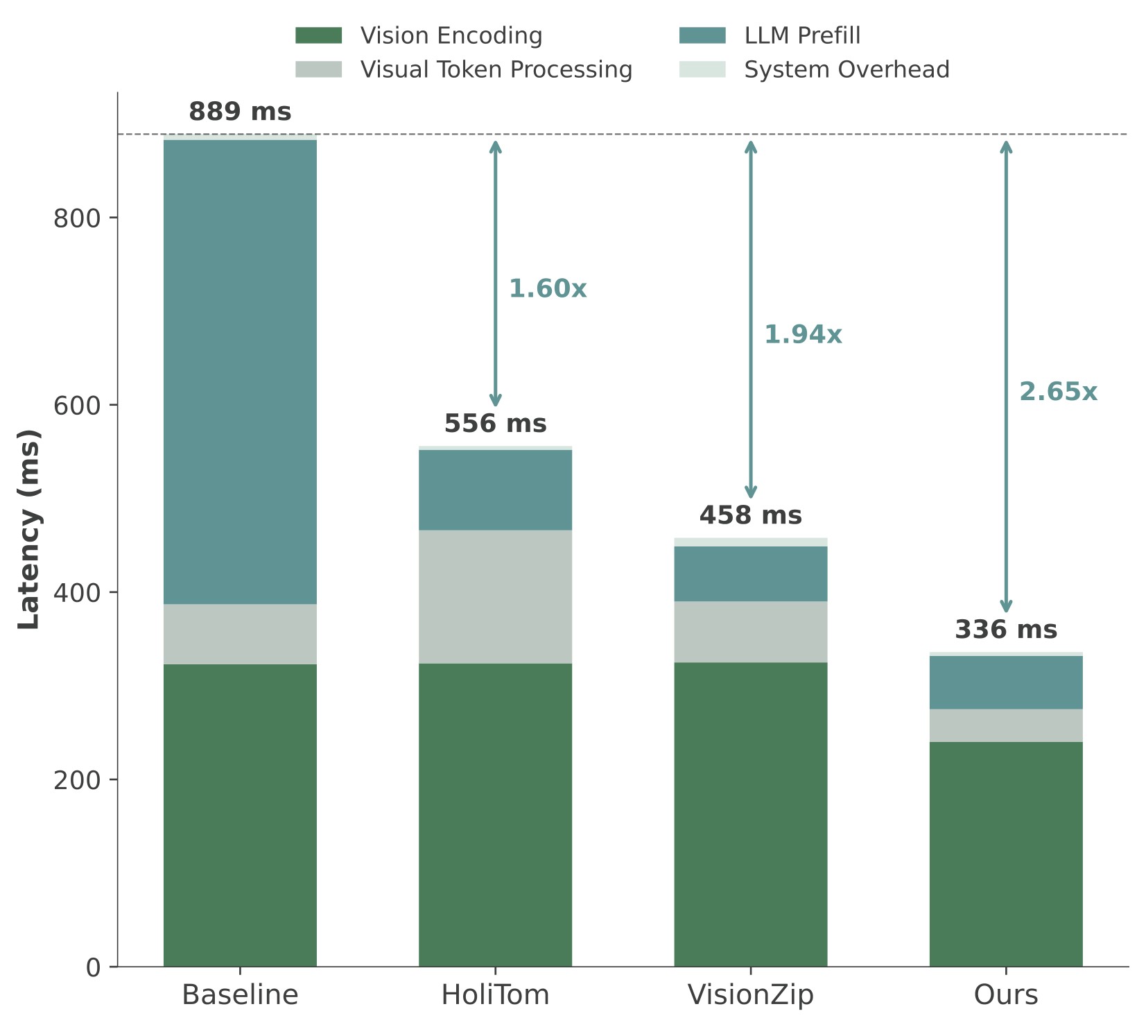
15%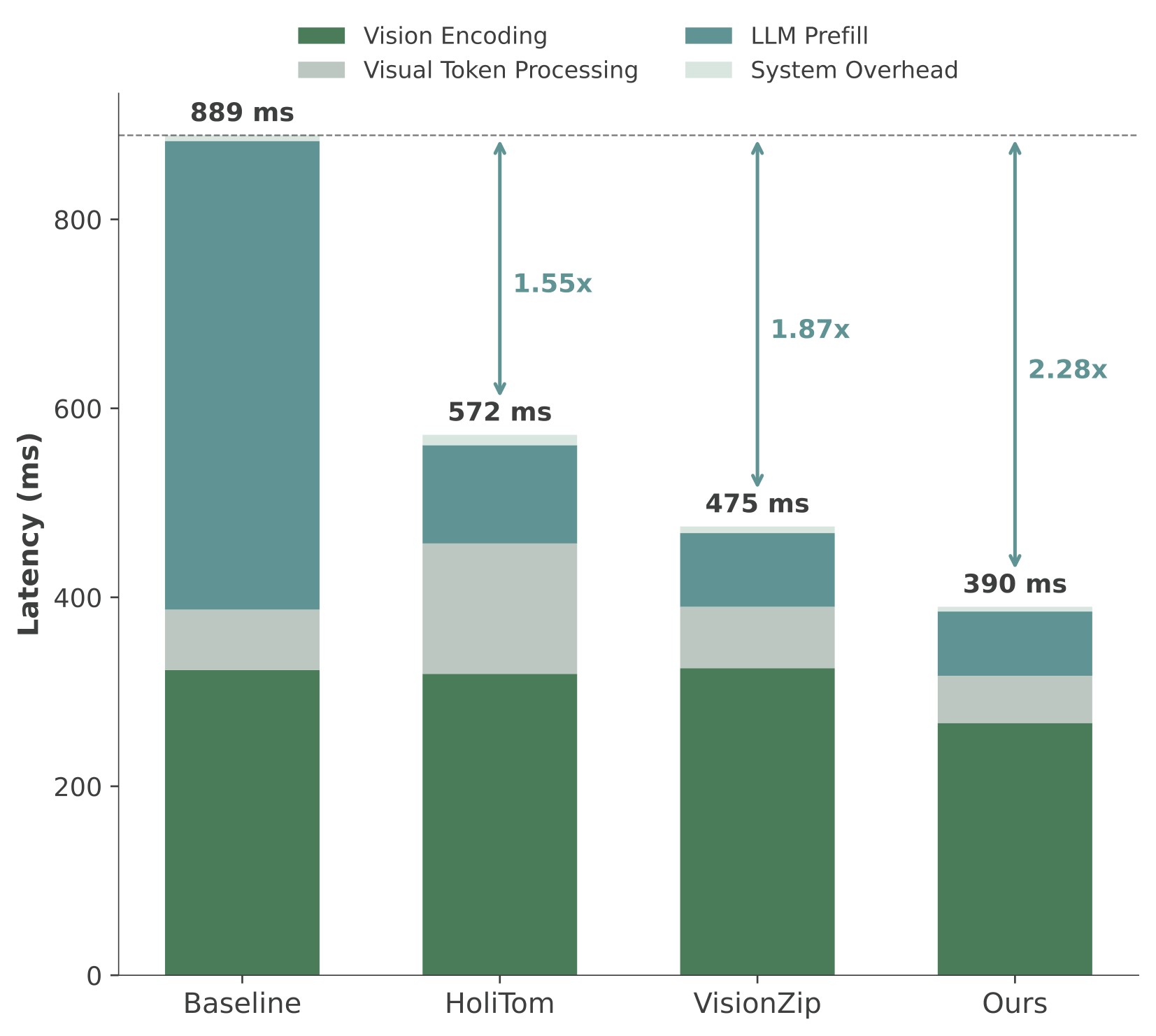
20%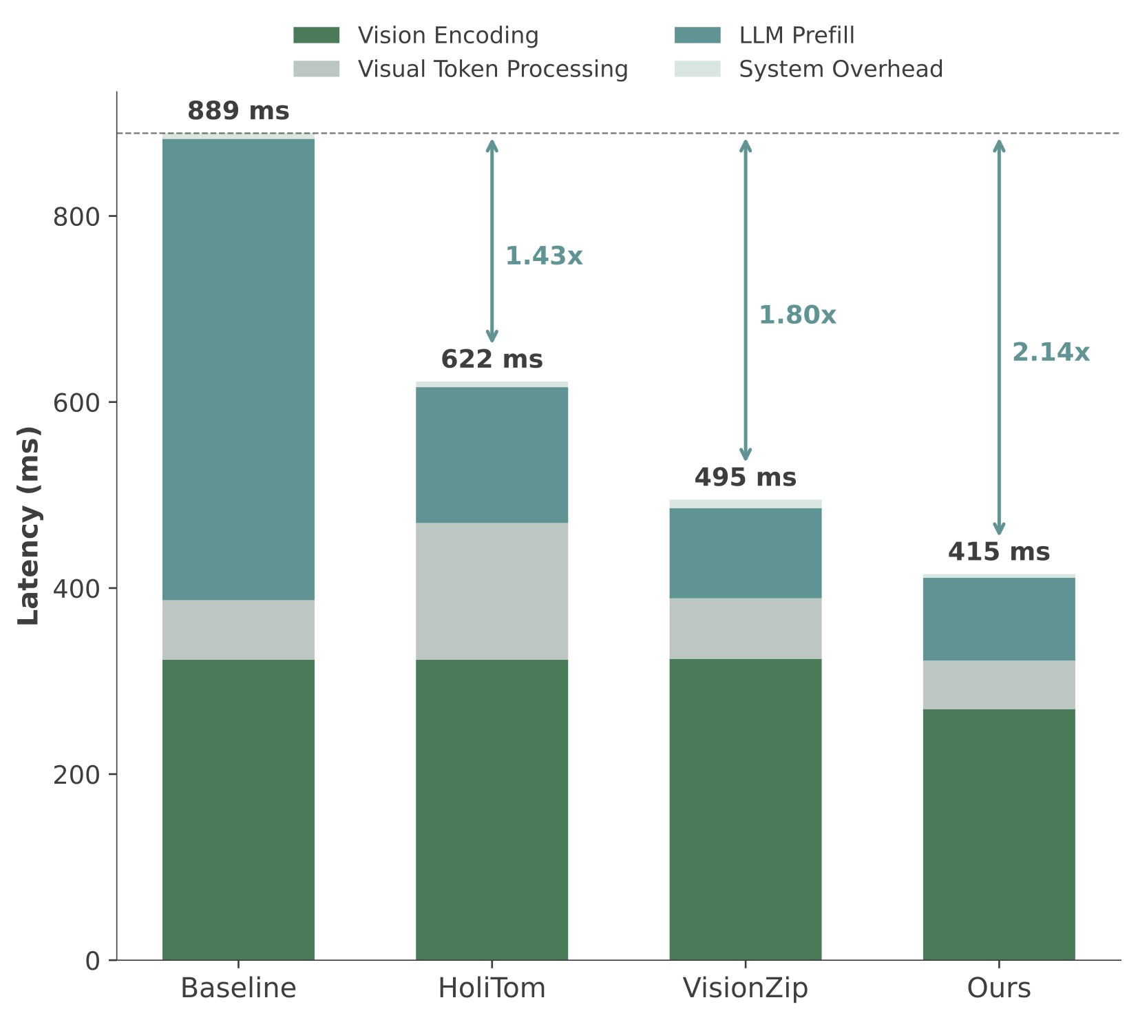
25%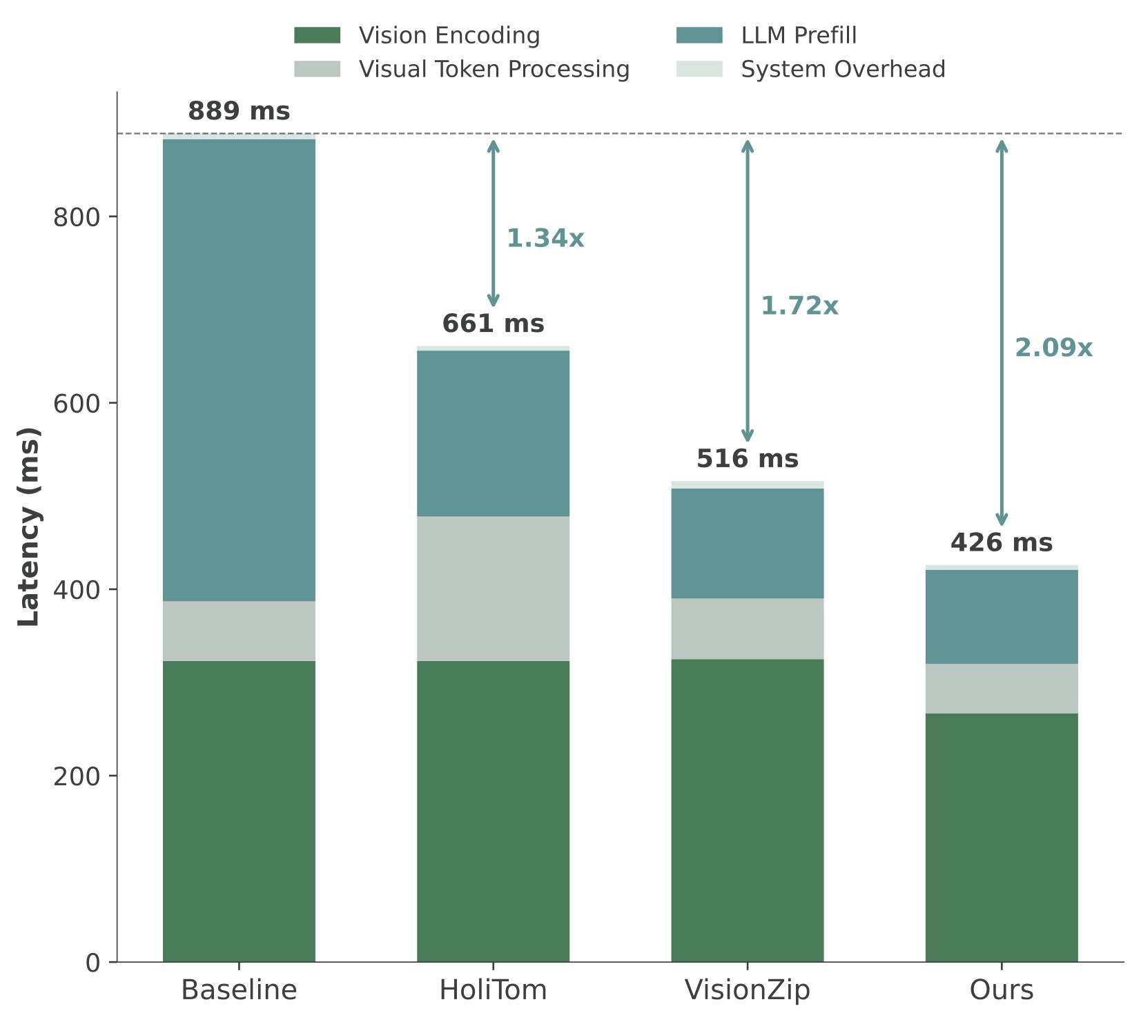

Figure 7. TTFT comparison on LLaVA-OneVision-7B. The source caption reports vision encoding, visual token processing, LLM prefill, and system overhead across methods. The paper states that EarlyTom has the lowest total TTFT across settings, with up to 2.65x speedup at 10% retention.

Figure 8 shows the same decomposition for the smaller 0.5B model.

0.5B retained ratio	Local figure
10%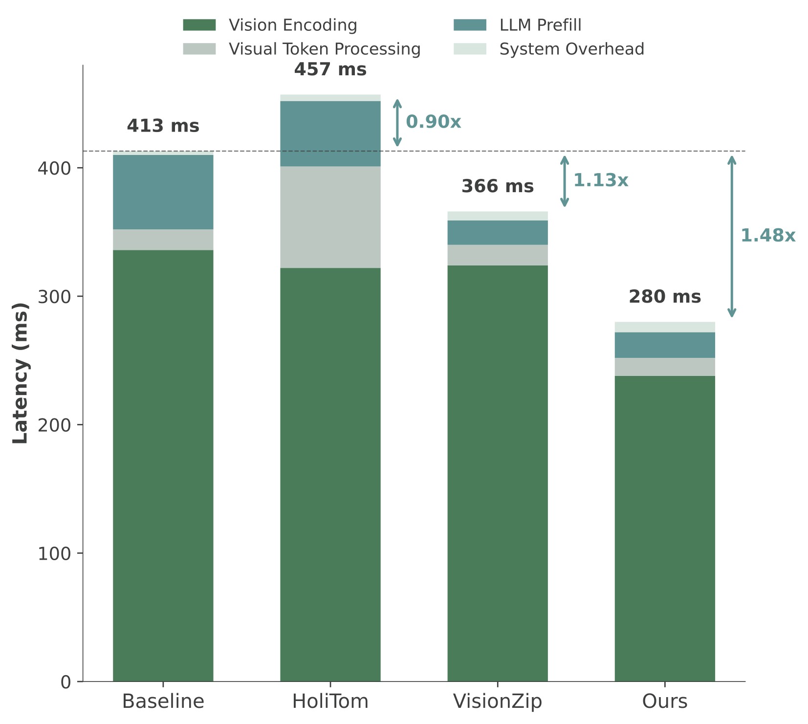
15%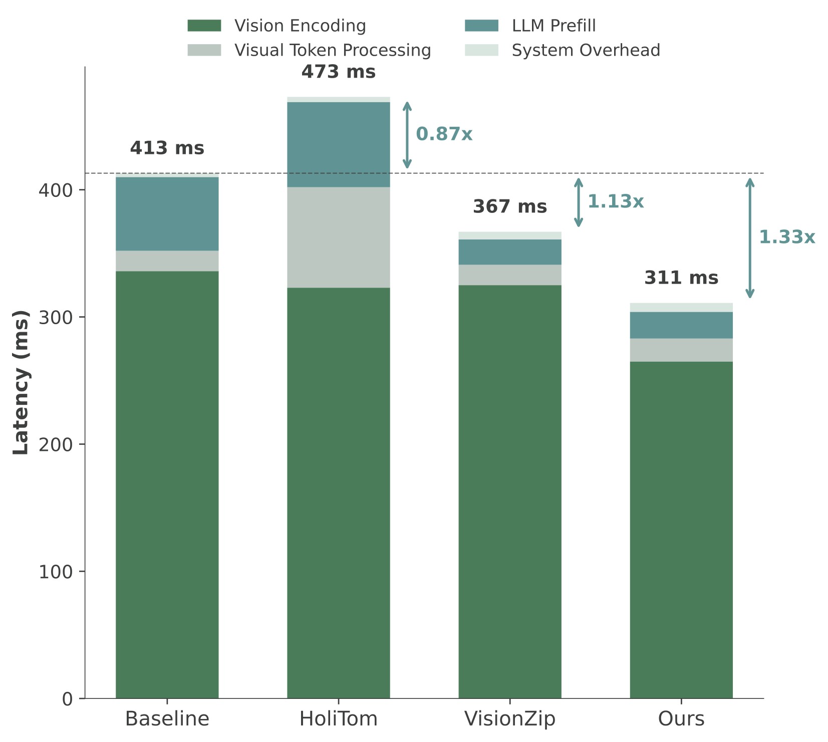
20%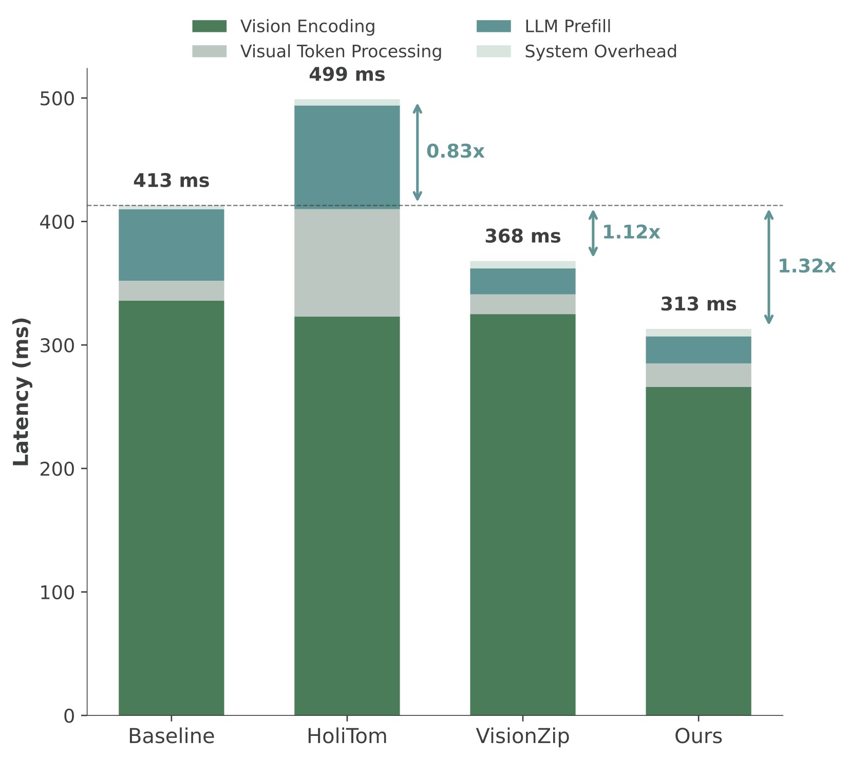
25%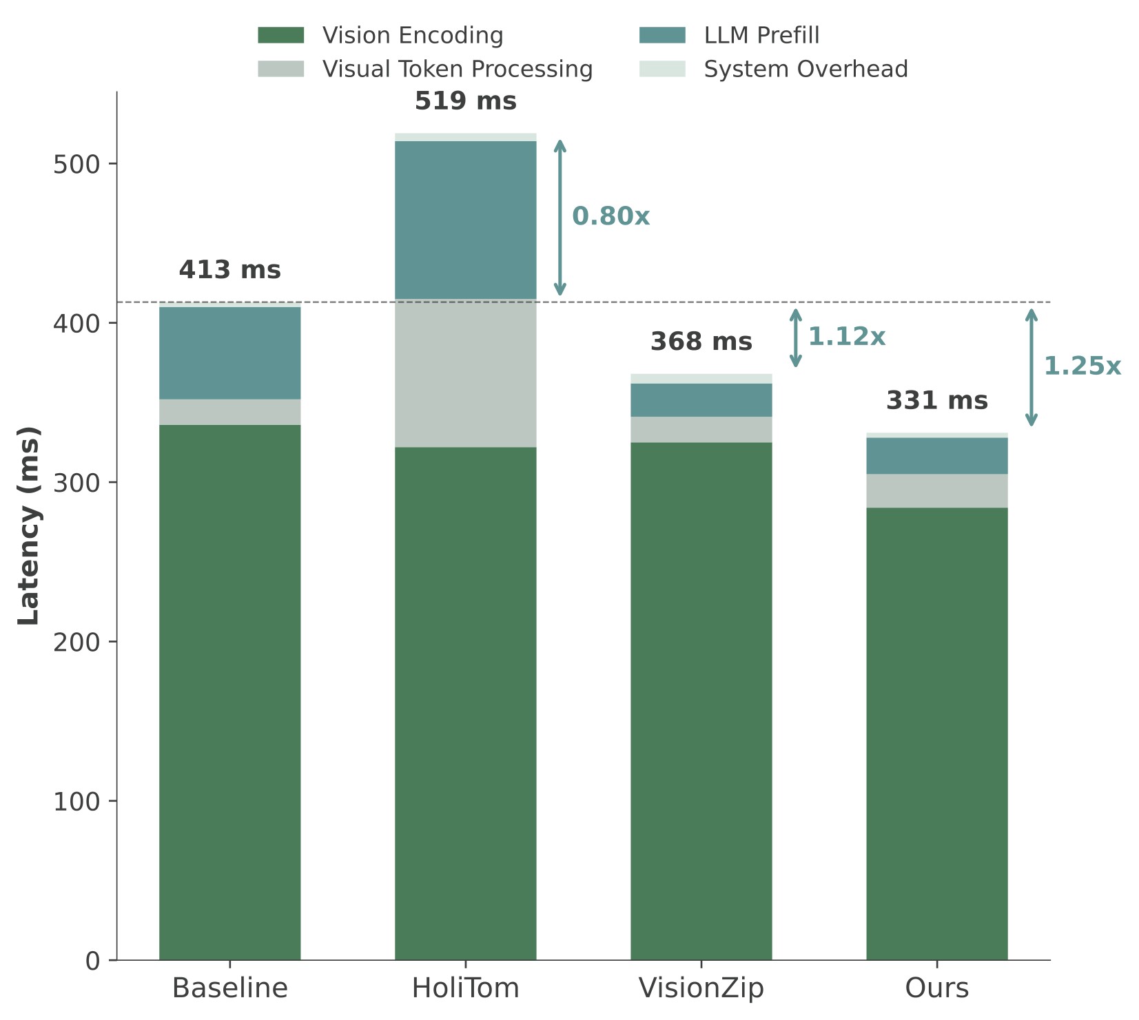

Figure 8. TTFT comparison on LLaVA-OneVision-0.5B. The source text highlights that HoliTom can be slower than the baseline on the 0.5B model at 10% retention, whereas EarlyTom keeps speedup by minimizing vision encoding time and extra processing overhead.

Practical Takeaways

The reusable idea is placement: compress before the vision encoder finishes processing every frame, not only after visual tokens are fully encoded.
The method is strongest as a serving-time intervention for Video-LLMs when TTFT matters. It is training-free in the source paper and evaluated with standard benchmark harnesses.
The attention-sink analysis matters. If token selection uses global attention scores without correction, static sink tokens can dominate retained visual positions; EarlyTom's dynamic/static split is a practical mitigation.
The best empirical evidence is the 7B LLaVA-OneVision table: EarlyTom reduces TTFT from 889.9 ms to 336.2 ms at 10% retention, while retaining 96.2% of average full-token benchmark performance.
The generalization evidence is credible but bounded. LLaVA-Video-7B and Qwen2.5-VL-7B results support the idea across backbones, but the method is still evaluated on selected Video-LLM stacks and benchmark suites.
The main weakness is that accuracy is not free at aggressive compression. On LLaVA-OneVision-7B, 10% EarlyTom drops the average score from 58.4 to 56.2; on LLaVA-Video-7B, EarlyTom has the best latency/FLOPs but not the best average score.

The paper's future-work section says EarlyTom mainly reveals that the inference budget is dominated by the prefill stage, and that broader heterogeneous system design plus decoding-stage acceleration remain open problems. For follow-up work, I would check whether the thresholds and layer choices transfer automatically to longer videos, different vision encoders, and more reasoning-heavy video tasks.