Source-first digest for checked paper rank 6, rank_id p012.
- Routing status:
success, but the Markdown manifest reports six missing main-text includes, so the main body was recovered from LaTeX source files rather than PDF extraction. - PDF extraction: not used
Motivation / Background
This paper asks whether VLM spatial-reasoning accuracy reflects structured 3D understanding or shortcut use from natural image statistics. The target shortcut is simple: in many photographs, objects that are farther away on the ground plane also appear higher in the image. A VLM can therefore answer "farther" questions by leaning on vertical image position instead of representing distance as its own spatial axis.
The authors call this failure mode vertical-distance entanglement. It matters for embodied and robotic settings because a model that appears good on standard spatial benchmarks may still fail when the natural correlation between "higher in the image" and "farther in 3D" is weakened, reversed, or synthetically controlled. Figure 1 summarizes the paper's thesis: many VLMs follow the perspective shortcut, while stronger spatial models separate axes and remain correct on counter-heuristic cases.
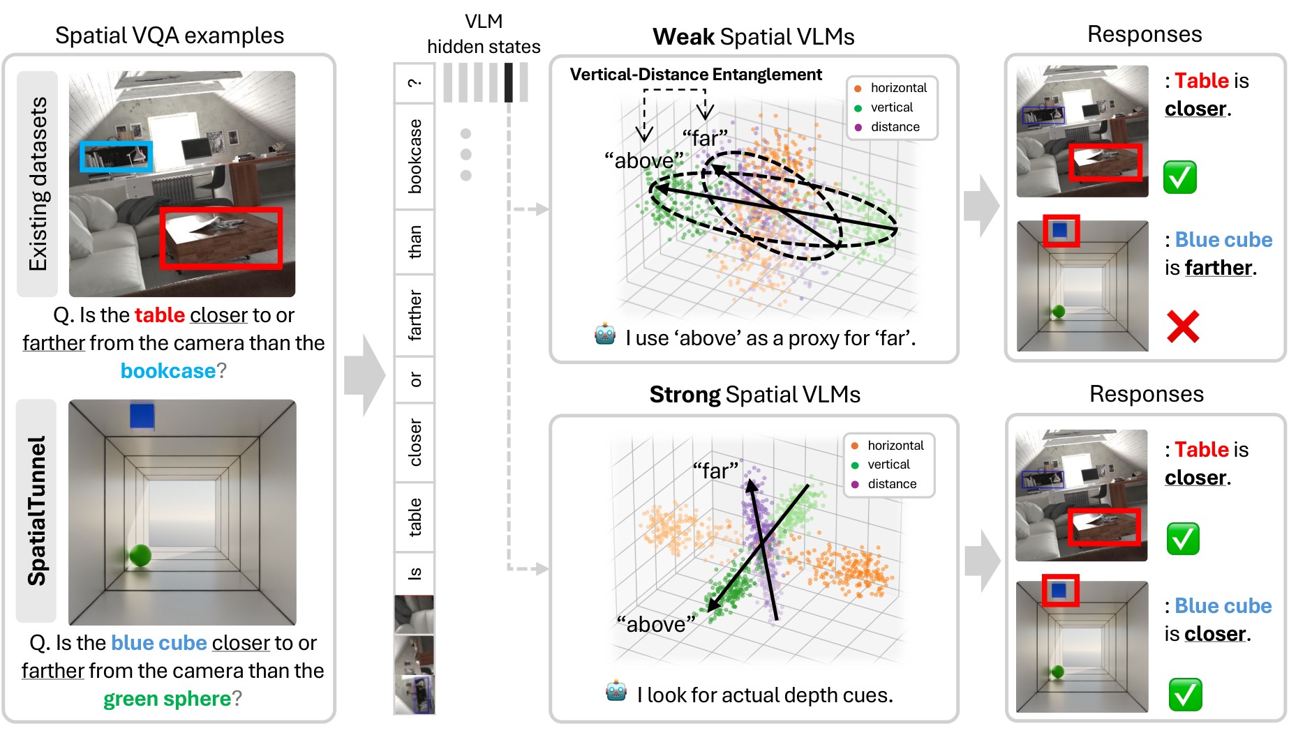
SpatialTunnel plus contrastive probing. I place it here because it is the clearest high-level statement of the paper's motivation and contribution.The geometric reason the shortcut exists is the standard ground-plane projection relation. For a camera at height \(H_c\) with focal length \(f\), a ground-plane point at depth \(Z\) projects to:
As \(Z\) grows, \(v_{\mathrm{img}}\) approaches the horizon, so farther ground-plane objects move upward in the image. The paper's core concern is that VLMs often internalize this correlation as if it were the depth relation itself.
Claims And Evidence
| Claim id | Main claim | Support | Evidence anchors |
|---|---|---|---|
| C1 | VLMs across multiple model families exhibit vertical-distance entanglement: they do better when the true depth relation agrees with the "higher means farther" heuristic than when it contradicts it. | 5 | problem overview, consistent/counter setup, real benchmark split, real accuracy, SpatialTunnel results |
| C2 | Existing real-image depth benchmarks are skewed toward perspective-consistent examples, so aggregate benchmark accuracy can overstate robust 3D reasoning. | 5 | distribution table, benchmark-performance table |
| C3 | SpatialTunnel isolates this shortcut by decoupling vertical image position from depth while keeping depth ordering fixed. |
4 | SpatialTunnel design, SpatialTunnel table, Molmo heatmaps |
| C4 | Spatial fine-tuning can improve average accuracy while still leaving distance representations weak or entangled; data scale alone is not a guarantee. | 4 | real accuracy, SpatialTunnel table, axis coherence |
| C5 | Contrastive probing gives a representation-level diagnostic: higher distance coherence and lower VD-EI align with better counter-heuristic robustness. | 4 | probing method, internal analysis, PCA, coherence table |
| C6 | Stronger spatial models such as RoboRefer and Qwen3-VL-235B have more separated spatial axes and stronger cross-benchmark performance. | 4 | spatial benchmarks, PCA, coherence table |
| C7 | Shortcut reliance is not limited to vertical image position; apparent size can create a similar depth cue failure. | 3 | object-size extension |
Scores are support-from-paper scores, not independent reproduction scores. C3-C6 are capped below 5 because the evidence is strong within the paper but still diagnostic/correlational rather than causal proof of the full training mechanisms.
Core Technical Idea
The paper combines two diagnostics:
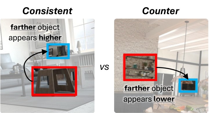
- A behavioral split that classifies depth questions as perspective-consistent or counter-heuristic depending on whether the farther object appears higher in the image.
- A representation probe that uses swapped question pairs to test whether the model's hidden-state deltas form separable horizontal, vertical, and distance axes.
The behavioral split asks whether the shortcut appears in outputs. The probing method asks whether the shortcut is geometrically present in representation space. This distinction is important: two models can have similar benchmark accuracy but very different internal spatial structure.
The consistent/counter categorization is visualized in Figure 2. This figure is referenced by the main text as the operational definition behind the real-benchmark and SpatialTunnel splits.
Method Details
Model And Data Setup
The experiments cover Molmo-7B-O-0924, NVILA-Lite-2B, Qwen2.5-VL-3B-Instruct, RoboRefer-2B-SFT, and Qwen3-VL-235B-A22B-Instruct. For Molmo, NVILA, and Qwen2.5-VL, the authors train spatial fine-tuning variants at 80k, 400k, 800k, and 2M samples. The sampled spatial data mix comes from SAT, RoboSpatial, SPAR-7M, RefSpatial, and PRISM. RoboRefer is treated as a depth/spatially supervised reference model sharing the NVILA base family, and Qwen3-VL-235B is treated as a very large-scale reference model.
Consistent-Counter Split
For real-image benchmarks, each depth-related example is grouped as:
- Consistent: the farther object has a smaller image \(y\)-coordinate, meaning it is higher in the image.
- Counter: the farther object appears lower.
- Ambiguous: the vertical center difference is too small to support a clean split.
The split is a behavioral test for whether models rely on the elevation cue. If a model truly reasons about 3D depth, consistent and counter accuracy should be close. Large positive gaps imply shortcut dependence.
SpatialTunnel
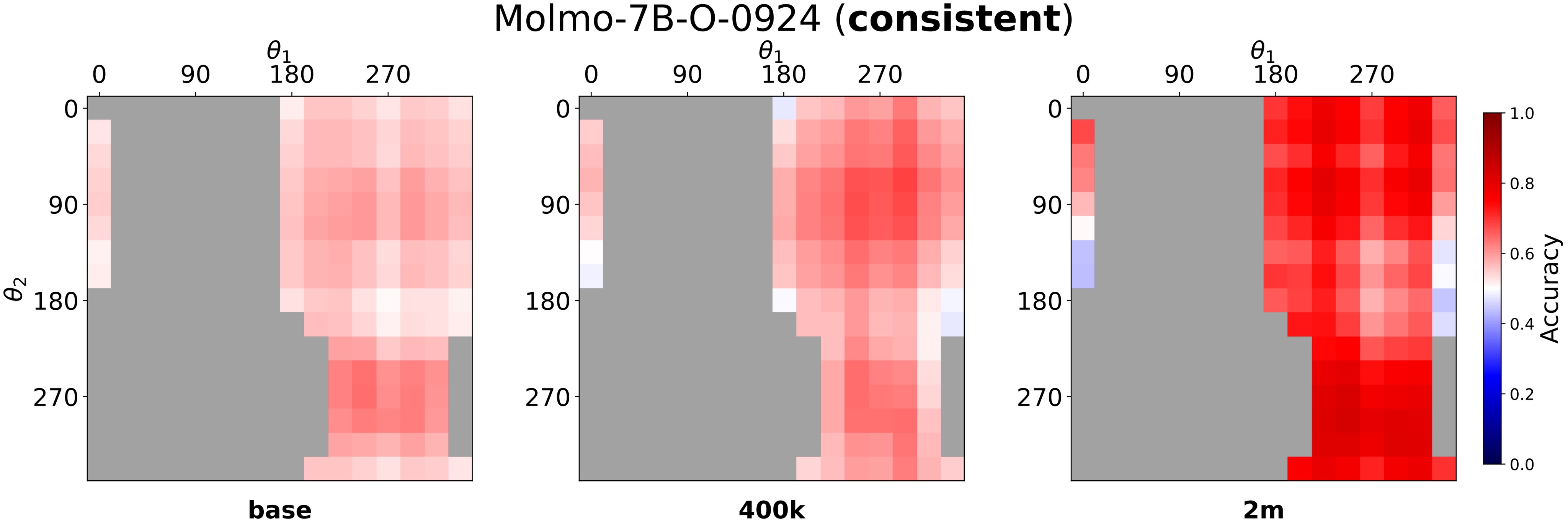
SpatialTunnel is a synthetic Blender benchmark built around a single-point-perspective corridor. Two objects are placed at fixed depths while their angular positions on the tunnel cross-section are swept independently. This creates a \(16 \times 16\) grid of positions where vertical image location changes without changing the true depth order. Figure 3 shows this design.

For each image, the model answers binary depth questions such as whether one object is closer or farther than the other. The probability-based scoring rule extracts the first-token logits for Yes and No:
The correctness score is \(v=p\) when the ground-truth answer is Yes, and \(v=1-p\) when it is No. Reported metrics are mean correctness \(v\), consistent correctness \(v_{\text{cons}}\), counter correctness \(v_{\text{ctr}}\), and the shortcut gap:
Contrastive Probing
Figure 6 summarizes the representation-level probe. For each VQA example, the authors build a minimally swapped question pair, such as "Is A left of B?" vs. "Is B left of A?", so the ground-truth spatial relation flips while the image and object identities remain fixed. They extract the final-token hidden state at an intermediate layer and compute the delta vector:
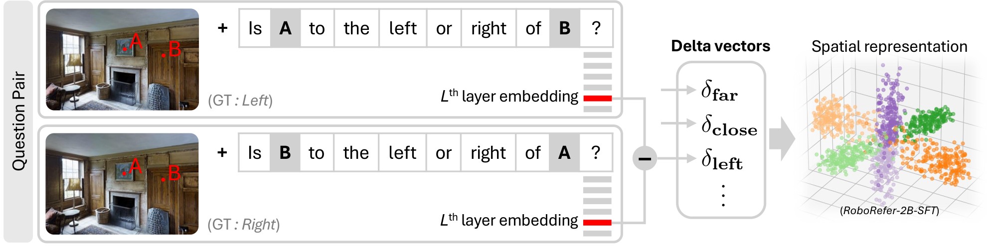
For each spatial axis, deltas from opposing categories are sign-corrected so they point in a canonical direction:
Axis coherence is then the mean pairwise cosine similarity over the sign-corrected set:
The vertical-distance entanglement index compares perspective-aligned and perspective-opposing mean deltas:
Positive VD-EI means the hidden representation aligns above with far and below with close.
Experiments And Results
Real Benchmark Evidence
Table 1 shows that real-image benchmarks are dominated by perspective-consistent examples. This supports C2: a model can receive a lot of credit on aggregate depth performance while repeatedly failing the rarer counter cases.
| Type | EmbSpatial-Bench | CV-Bench-3D | Definition |
|---|---|---|---|
| Consistent | 976 (80.9%) | 363 (60.5%) | Ground truth aligns with heuristic |
| Counter | 129 (10.7%) | 65 (10.8%) | Ground truth contradicts heuristic |
| Ambiguous | 101 (8.4%) | 172 (28.7%) | Vertical difference below 5% of image height |
Table 1. Distribution of consistent, counter, and ambiguous examples. The skew toward consistent examples mirrors natural perspective statistics.
Table 2 is the main real-image evidence for C1. Every listed model family has lower counter accuracy than consistent accuracy. The most striking example is Qwen2.5-VL-3B with 2M spatial samples: 60.9% consistent vs. 24.0% counter on EmbSpatial-Bench.
| Model | EmbSpatial Consistent | EmbSpatial Counter | CV-3D Consistent | CV-3D Counter |
|---|---|---|---|---|
| Molmo-7B-O-0924 | 63.5 | 34.9 | 93.1 | 75.4 |
| + 80k | 60.6 | 29.5 | 80.2 | 56.9 |
| + 400k | 62.7 | 27.1 | 89.5 | 56.9 |
| + 800k | 65.2 | 34.1 | 88.7 | 70.8 |
| + 2M | 65.3 | 39.5 | 90.6 | 72.3 |
| NVILA-Lite-2B | 49.0 | 27.1 | 74.4 | 40.0 |
| + 80k | 57.7 | 15.5 | 71.6 | 50.8 |
| + 400k | 61.1 | 34.1 | 81.3 | 58.5 |
| + 800k | 63.2 | 38.8 | 84.6 | 67.7 |
| + 2M | 60.7 | 41.1 | 97.2 | 93.8 |
| RoboRefer-2B-SFT | 87.0 | 59.7 | 98.9 | 95.4 |
| Qwen2.5-VL-3B | 54.7 | 32.6 | 75.5 | 55.4 |
| + 80k | 50.6 | 30.2 | 69.7 | 60.0 |
| + 400k | 52.6 | 27.1 | 65.8 | 58.5 |
| + 800k | 55.8 | 26.4 | 61.2 | 58.5 |
| + 2M | 60.9 | 24.0 | 62.0 | 53.8 |
| Qwen3-VL-235B | 73.3 | 41.7 | 98.1 | 90.8 |
Table 2. Accuracy on consistent vs. counter examples. Values are accuracies from depth-related examples in EmbSpatial-Bench and CV-Bench-3D. The gap persists across architectures, scales, and fine-tuning levels.
SpatialTunnel Evidence
Table 3 confirms the same pattern in a controlled synthetic environment. Because SpatialTunnel balances the geometry and decouples vertical position from depth, the positive \(\Delta\) values are stronger evidence that the shortcut is model-intrinsic rather than merely a property of evaluation-set skew.
| Model | \(v\) | \(v_{\text{cons}}\) | \(v_{\text{ctr}}\) | \(\Delta\) |
|---|---|---|---|---|
| Molmo-7B-O-0924 | 0.528 | 0.565 | 0.487 | +0.078 |
| + 80k | 0.496 | 0.507 | 0.486 | +0.021 |
| + 400k | 0.501 | 0.593 | 0.409 | +0.184 |
| + 800k | 0.531 | 0.628 | 0.430 | +0.198 |
| + 2M | 0.666 | 0.703 | 0.630 | +0.073 |
| NVILA-Lite-2B | 0.488 | 0.504 | 0.471 | +0.033 |
| + 80k | 0.499 | 0.562 | 0.438 | +0.124 |
| + 400k | 0.669 | 0.804 | 0.538 | +0.267 |
| + 800k | 0.646 | 0.728 | 0.571 | +0.157 |
| + 2M | 0.812 | 0.875 | 0.749 | +0.127 |
| RoboRefer-2B-SFT | 0.793 | 0.816 | 0.770 | +0.046 |
| Qwen2.5-VL-3B | 0.570 | 0.776 | 0.360 | +0.416 |
| + 80k | 0.512 | 0.585 | 0.440 | +0.145 |
| + 400k | 0.503 | 0.588 | 0.418 | +0.171 |
| + 800k | 0.499 | 0.600 | 0.398 | +0.202 |
| + 2M | 0.500 | 0.648 | 0.353 | +0.295 |
| Qwen3-VL-235B | 0.908 | 0.948 | 0.880 | +0.068 |
Table 3. Consistent vs. counter correctness on SpatialTunnel. \(v\) is mean correctness, \(v_{\text{cons}}\) is correctness on consistent samples, \(v_{\text{ctr}}\) is correctness on counter samples, and \(\Delta\) is their difference.
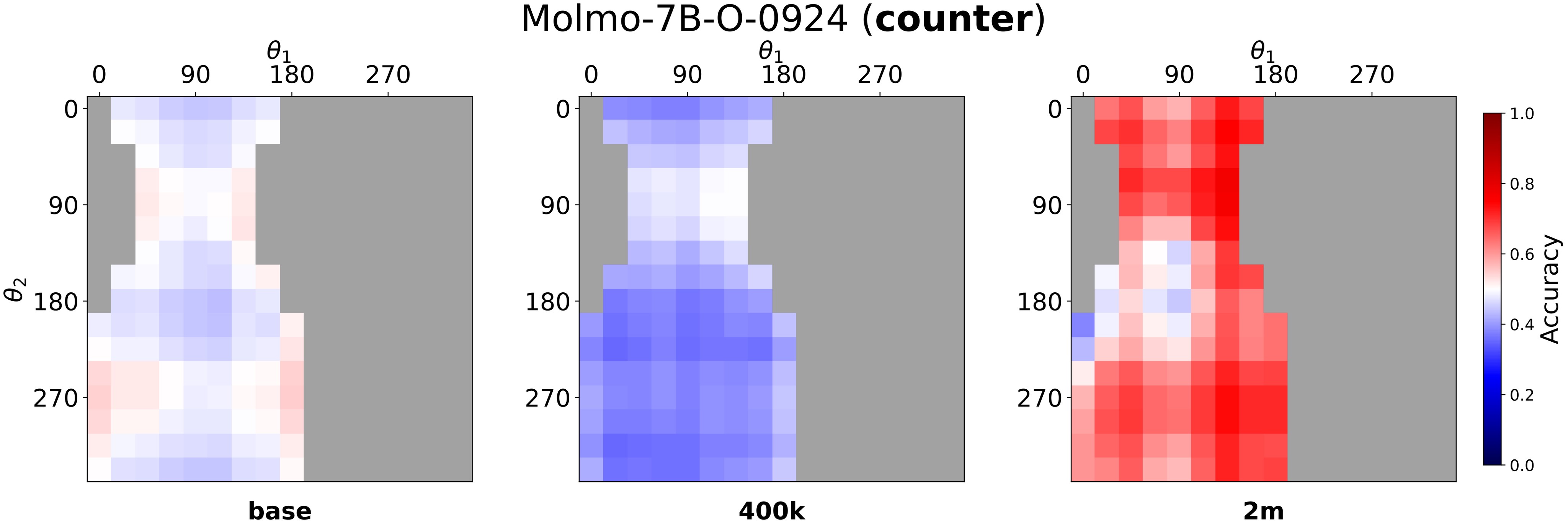
The Molmo heatmaps in Figure 4 and Figure 5 show the spatial pattern behind the aggregate scores. Consistent cells become easier with scaling, while counter cells remain harder and are especially degraded around intermediate fine-tuning steps.
Benchmark Accuracy Is Not Enough
Table 4 broadens the evaluation across EmbSpatial, CV-Bench, and BLINK. The pattern is not a clean "more spatial fine-tuning means better spatial understanding" story. For example, NVILA 2M reaches 93.8 on CV-3D Depth but only 62.9 on BLINK Spatial Relation, while Qwen 2M is 78.3 on BLINK Spatial Relation but 52.2 on CV-3D Distance.
| Model | EmbSpatial Overall | CV-2D Relation | CV-3D Depth | CV-3D Distance | BLINK Rel. Depth | BLINK Spat. Rel. |
|---|---|---|---|---|---|---|
| Molmo-7B-O-0924 | 60.7 | 76.3 | 84.5 | 68.5 | 78.2 | 70.6 |
| + 80k | 52.9 | 62.3 | 71.0 | 67.5 | 72.6 | 60.8 |
| + 400k | 64.9 | 84.3 | 80.0 | 70.8 | 72.6 | 68.5 |
| + 800k | 69.1 | 90.0 | 82.0 | 70.8 | 75.0 | 61.5 |
| + 2M | 74.3 | 93.7 | 87.3 | 81.3 | 71.0 | 69.2 |
| NVILA-Lite-2B | 54.0 | 58.6 | 69.2 | 52.3 | 64.5 | 67.1 |
| + 80k | 65.1 | 78.9 | 66.2 | 60.8 | 53.2 | 74.1 |
| + 400k | 62.1 | 83.2 | 74.3 | 67.0 | 71.8 | 63.6 |
| + 800k | 69.7 | 85.5 | 78.2 | 71.3 | 57.3 | 65.0 |
| + 2M | 69.4 | 91.4 | 93.8 | 87.2 | 70.2 | 62.9 |
| RoboRefer-SFT-2B | 92.0 | 96.5 | 95.7 | 90.5 | 84.7 | 79.7 |
| Qwen2.5-VL-3B | 62.3 | 67.4 | 70.3 | 60.2 | 68.6 | 83.9 |
| + 80k | 57.3 | 59.7 | 64.7 | 61.5 | 58.1 | 79.7 |
| + 400k | 58.6 | 58.2 | 62.0 | 54.5 | 58.9 | 78.3 |
| + 800k | 60.9 | 59.4 | 58.7 | 51.2 | 58.1 | 79.0 |
| + 2M | 65.7 | 68.8 | 58.5 | 52.2 | 53.2 | 78.3 |
| Qwen3-VL-235B | 82.0 | 96.5 | 93.3 | 91.0 | 84.7 | 90.2 |
Table 4. Performance across spatial benchmarks. Fine-tuned variants fluctuate across benchmark formats. RoboRefer and Qwen3-VL-235B are more consistently strong.
Representation-Level Evidence
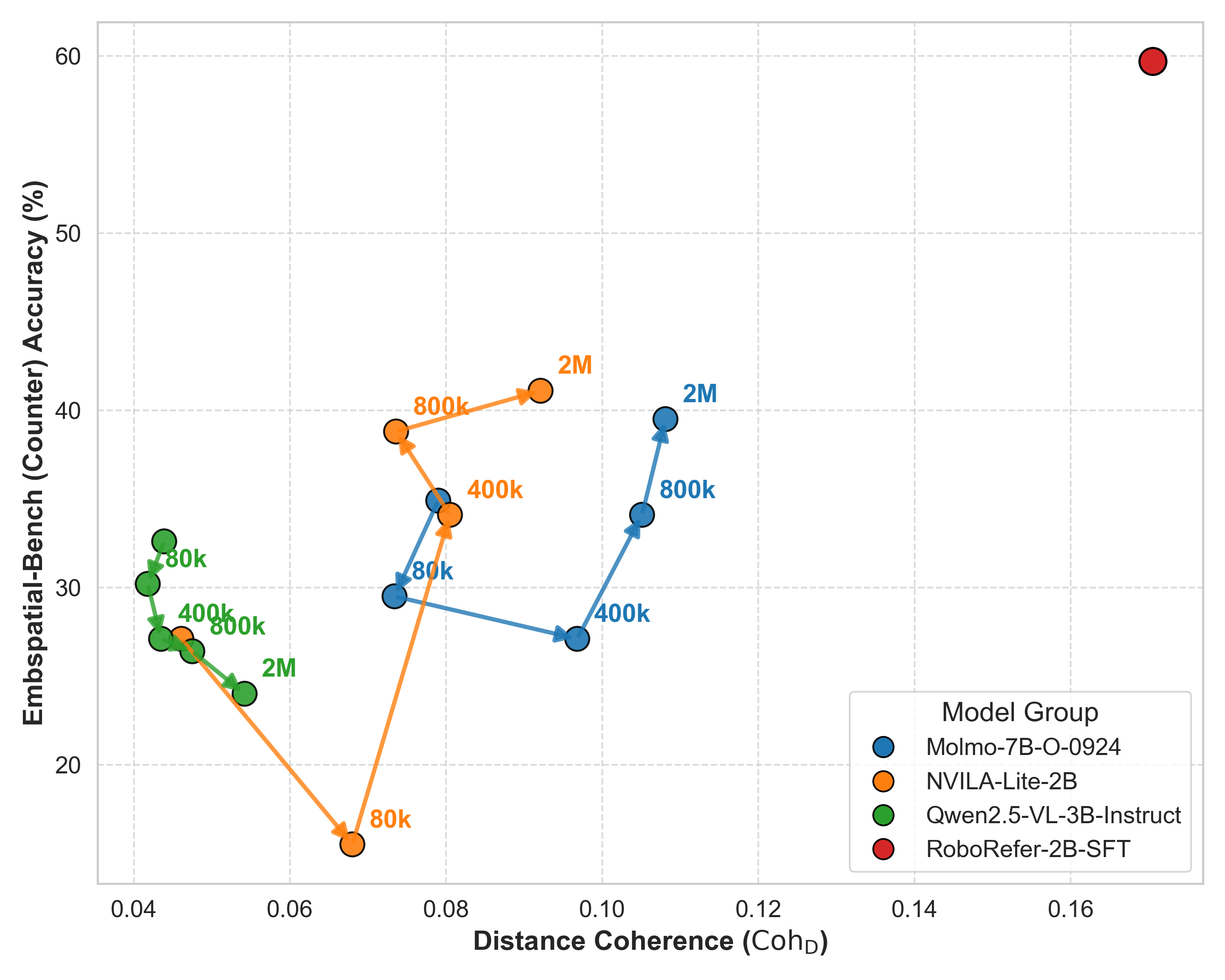
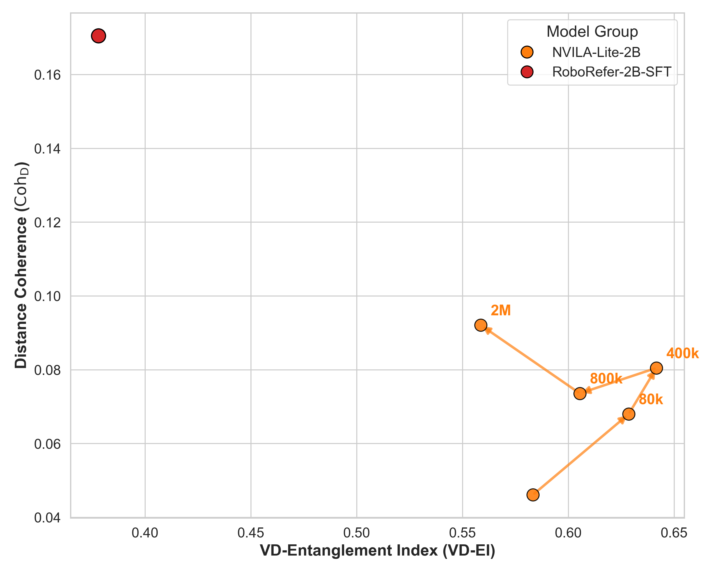
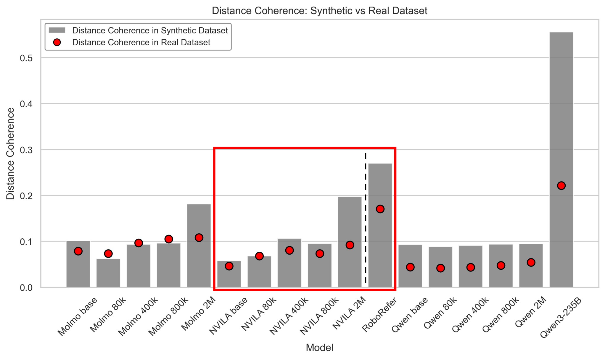
Figure 7 links counter accuracy to distance coherence. The paper reports that \(\mathrm{Coh}_D\) computed on SpatialTunnel correlates with counter accuracy on EmbSpatial-Bench and CV-Bench-3D with Spearman \(\rho=0.759\) and \(\rho=0.804\), respectively, both with \(p<10^{-3}\). Figure 8 shows that within the NVILA family, RoboRefer occupies the desirable region of high distance coherence and lower VD-EI.
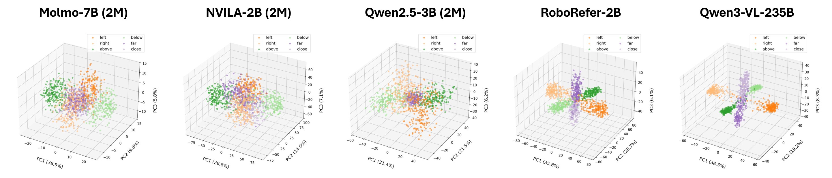
The PCA visualization in Figure 9 makes the same point visually. Molmo 2M, NVILA 2M, and Qwen 2M separate horizontal and vertical deltas better than distance deltas; RoboRefer and Qwen3 show much cleaner separation of all three axes.
| Model | \(\mathrm{Coh}_H\) | \(\mathrm{Coh}_V\) | \(\mathrm{Coh}_D\) | VD-EI |
|---|---|---|---|---|
| Molmo-7B | 0.143 | 0.228 | 0.075 | 0.279 |
| + 80k | 0.122 | 0.332 | 0.072 | 0.388 |
| + 400k | 0.236 | 0.597 | 0.096 | 0.459 |
| + 800k | 0.247 | 0.559 | 0.107 | 0.514 |
| + 2M | 0.239 | 0.574 | 0.112 | 0.474 |
| NVILA-2B | 0.323 | 0.289 | 0.052 | 0.539 |
| + 80k | 0.295 | 0.497 | 0.070 | 0.606 |
| + 400k | 0.242 | 0.574 | 0.095 | 0.589 |
| + 800k | 0.278 | 0.498 | 0.089 | 0.591 |
| + 2M | 0.241 | 0.553 | 0.104 | 0.550 |
| RoboRefer-2B | 0.649 | 0.830 | 0.182 | 0.362 |
| Qwen2.5-3B | 0.367 | 0.293 | 0.043 | 0.457 |
| + 80k | 0.386 | 0.315 | 0.040 | 0.456 |
| + 400k | 0.450 | 0.452 | 0.042 | 0.451 |
| + 800k | 0.473 | 0.538 | 0.045 | 0.429 |
| + 2M | 0.485 | 0.586 | 0.052 | 0.472 |
Table 5. Axis coherence and VD-Entanglement Index. Distance coherence is the weakest axis across the reported models. RoboRefer has the highest coherence on all three axes and lower VD-EI than the NVILA scaling variants.
Additional Evidence From Source Appendices
The appendix extends the cue analysis from vertical position to object size. Figure 10 shows that Molmo and NVILA degrade when the farther object becomes larger than the nearer object, while Qwen remains near chance and therefore cannot be read as robust. This supports C7: high average depth accuracy can reflect multiple correlated visual cues, not just true 3D reasoning.
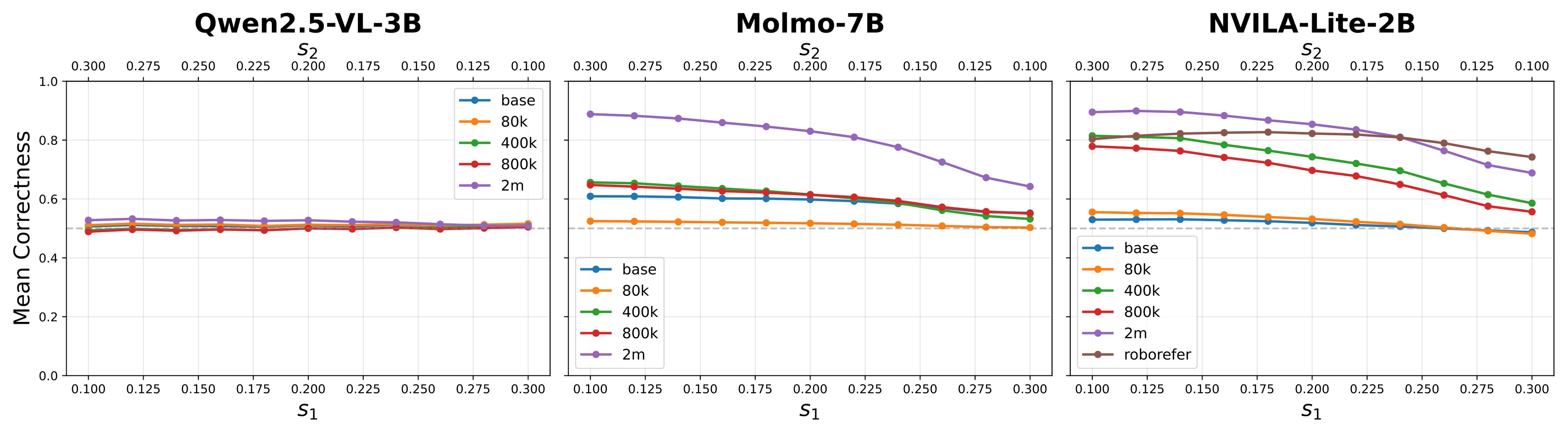
Figure 11 is useful as an externality check on the probing metric: the absolute \(\mathrm{Coh}_D\) values differ between synthetic SpatialTunnel and real EmbSpatial-Bench, but the relative ordering within model families is largely preserved.
Practical Takeaways
- The main reusable idea is the split between behavior and representation: benchmark accuracy says whether a model answered correctly, while contrastive probing asks whether it encoded spatial axes cleanly.
- The highest-value diagnostic is distance coherence. In this paper, \(\mathrm{Coh}_D\) is consistently the weakest axis and tracks counter-heuristic robustness better than aggregate accuracy alone.
- Spatial fine-tuning is not automatically enough. Some fine-tuned variants improve benchmark scores while maintaining or increasing shortcut gaps.
- RoboRefer and Qwen3-VL-235B are the strongest evidence that better spatial representations are possible, but the paper does not isolate a single causal ingredient; RoboRefer differs in both data scale and supervision, and Qwen3 differs heavily in model scale.
- The limitation to remember is that
SpatialTunnelis synthetic and diagnostic. It isolates one failure mode well, but it is not a full proxy for embodied 3D competence. - For future model evaluation, the paper argues for reporting counter-heuristic splits and representation structure, not only standard benchmark averages.