Why Larger Models Learn More: Effects of Capacity, Interference, and Rare-Task Retention

Source-first digest for checked paper rank 55, rank_id p033.

Routing status: pandoc_failed
PDF extraction: not used

Motivation / Background

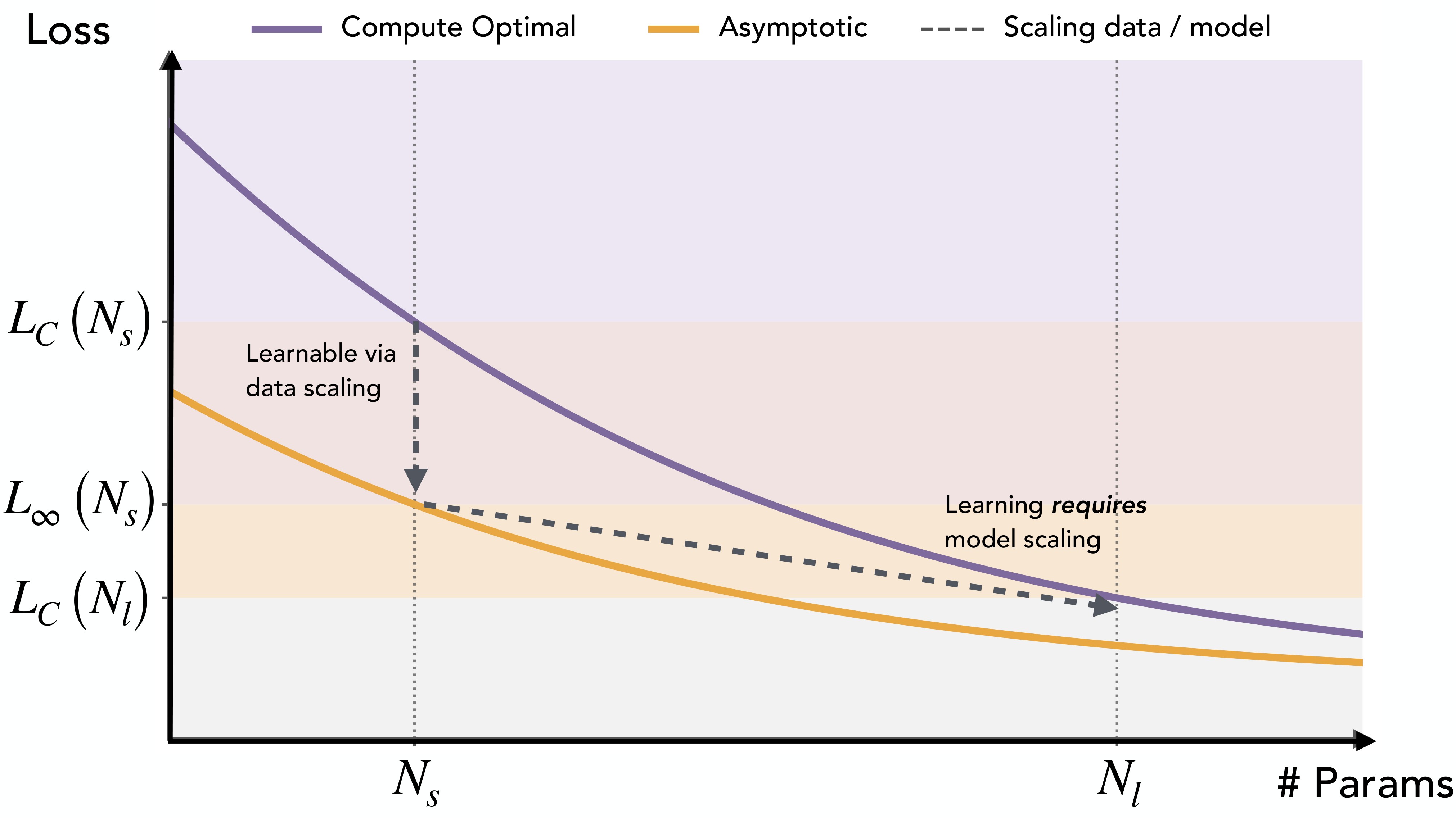
The paper asks a narrow but important scaling question: when a larger model succeeds on a task that a smaller model misses, is the smaller model merely undertrained, or is there a part of the data mixture that cannot be learned without increasing model capacity? The authors argue that standard power-law scaling already suggests a regime where extra data alone cannot recover the loss reached by a larger model, then use controlled task mixtures to study what that missing part of the distribution looks like.

Their answer is data-centric rather than purely expressivity-centric. Smaller models allocate limited representational directions to high-frequency or low-complexity tasks, so low-frequency or high-complexity tasks are not retained long enough to accumulate into generalizable structure. Larger models have enough width to explain common tasks, which weakens common-task gradients and reduces interference against rare-task updates. The conceptual distinction between "learnable via data scaling" and "learned via model scaling" is summarized in Figure 1.

**Figure 1. Learning a part of the distribution requires model scaling.** The original caption contrasts loss recovered by more data with loss that remains inaccessible to a smaller model even under asymptotic data scaling. I place it here because it motivates the paper's core category: capabilities or distributional regions that require model scaling, not just more samples.

Claims And Evidence

The support ratings in Table 1 are support-from-paper scores, not independent reproduction scores.

Claim id	Main claim	Support	Evidence anchors
C1	Power-law scaling motivates a regime where model scaling explains part of the data distribution that data scaling alone cannot recover for a smaller model.	3	conceptual scaling argument, limitations
C2	In the synthetic mixture, a width-\(N\) model learns the top-\(N\) task features by utility \(u_{k,j} = \pi_k \lambda_{k,j}\), so rare or complex tasks require larger width.	5	utility theorem, phase diagram, long-horizon check
C3	Larger width reduces interference from common tasks and lets rare-task updates persist between sparse observations.	5	gradient bound, residual control, rare-task retention
C4	The same rare-task pattern appears in an OLMo-style pretraining pipeline with injected comparison and modular-addition tasks.	4	OLMo setup, OLMo phase diagrams, injection-gap evidence
C5	Larger OLMo models embed more task-relevant features and show less gradient interference on localized task neurons.	4	representational evidence, gradient evidence
C6	Practically, increasing target-task frequency or managing data-mixture interference may sometimes be a more efficient route than only increasing parameters.	3	task-vs-LM loss, compute comparison, discussion and limitations

Core Technical Idea

The paper separates three explanations for why larger models do better:

Expressivity: the small model cannot represent the solution.
Sample efficiency: the small model could learn it, but needs more data or compute.
Data-mixture learning dynamics: the small model has enough formal expressivity for the task, but gradient-based training on a mixture allocates scarce representational resources to higher-utility tasks.

The authors focus on the third explanation. Their synthetic setting is a mixture of linear regression tasks. Task \(k\) appears with frequency \(\pi_k\) and has covariance spectrum \(C_k = B_k \Lambda_k B_k^\top\), where larger or slower-decaying spectra represent more complex tasks. The student has a shared width-\(N\) encoder and task-specific linear decoders.

The central capacity theorem says the mixture loss reduces to an eigenspace problem:

L_N(U) = \mathrm{tr}(M) - \mathrm{tr}(U^\top M U), \qquad M = \sum_{k=1}^{K} \pi_k C_k.

The retained features are ranked by per-feature utility:

u_{k,j} := \pi_k \lambda_{k,j}.

A width-\(N\) minimizer spans the top-\(N\) eigenspace of \(M\). If \(n_k(N)\) features from task \(k\) are retained, then the task's remaining loss is:

\ell_k^*(N) = \sum_{j>n_k(N)} \lambda_{k,j}.

This gives a concrete answer to "what does width buy?" It buys lower-utility features: rare tasks have low \(\pi_k\), complex tasks spread mass over many \(\lambda_{k,j}\), and both are postponed until the representation has enough capacity.

The second technical step explains why a rare task can be observed and still forgotten. Let \(\mathcal{F}\) be the frequent-task set, \(M_{\mathcal{F}} = \sum_{k \in \mathcal{F}} \pi_k C_k\), and \(\delta_{\mathcal{F}}(U)=\mathrm{tr}((I-P_U)M_{\mathcal{F}})\) be the remaining frequent-task residual. The common-task gradient obeys:

\|G_{\mathcal{F}}(U)\|_F \le 2\sqrt{\lambda_1(M_{\mathcal{F}})\,\delta_{\mathcal{F}}(U)}.

Once a model has enough width to explain common tasks, their residual drops, their gradient pressure weakens, and rare-task directions can persist. For a rare rank-one task \(C_r=\lambda_r b_r b_r^\top\), the paper also gives a critical-width condition:

N_r^{\mathrm{crit}} = \min\{N : \mu_N^{\mathcal{F}} \le \pi_r \lambda_r\}.

Below that width, the rare feature may be briefly learned after an injection batch but is eventually displaced by a common-task feature with higher utility.

Method Details

Synthetic Task Mixture

The synthetic experiments use \(K=32\) linear regression tasks in mutually orthogonal feature blocks. Task frequencies follow a power law \(k^{-\beta}\), and task spectra use power-law decay. The teacher for task \(k\) is:

y_k = \Lambda_k^{1/2}B_k^\top x.

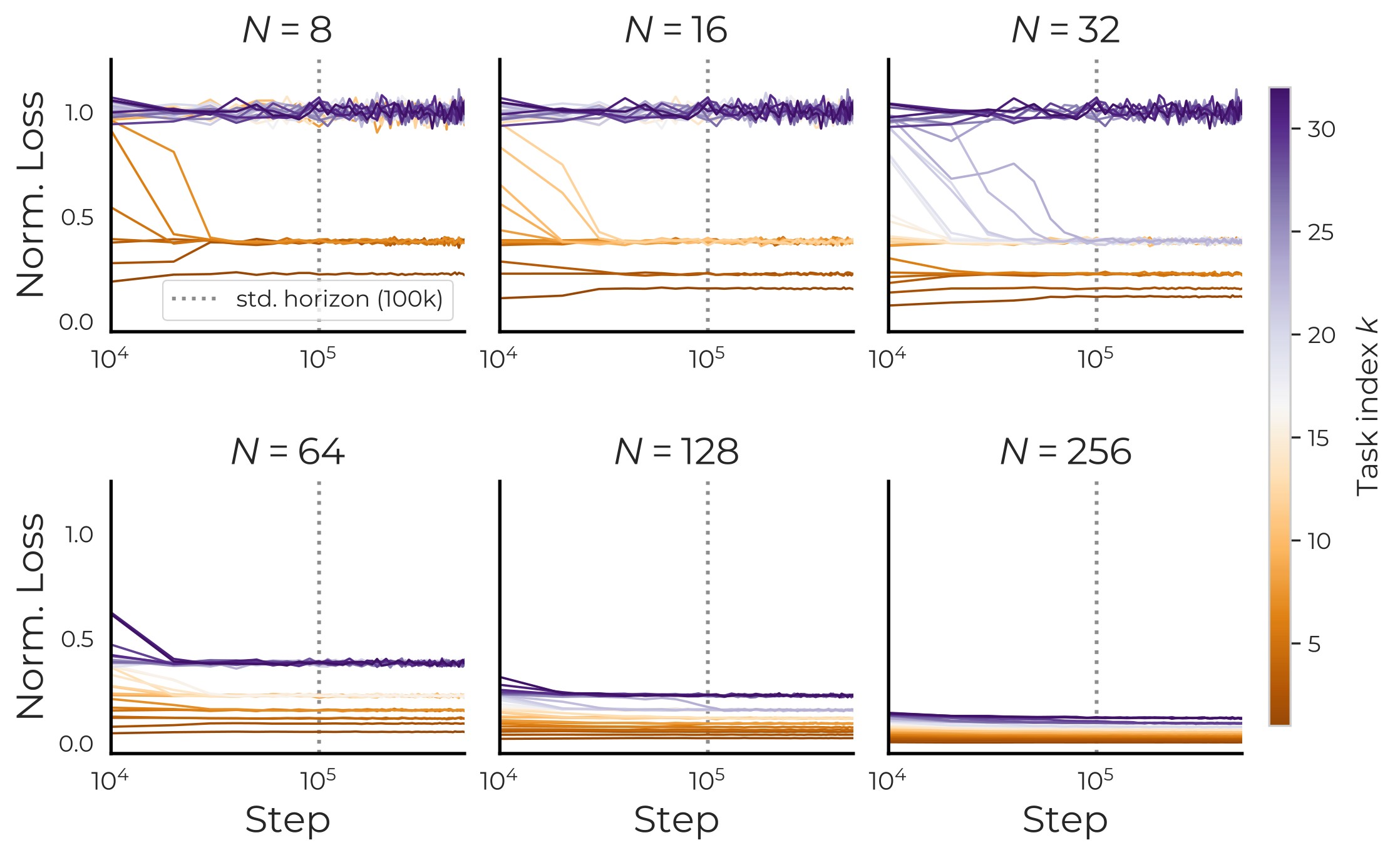
The student uses a shared encoder \(U\) and task-specific decoders \(D_k\), with prediction \(\hat{y}_k = D_k U^\top x\). Most phase-diagram runs train for 100K steps with Adam; the appendix extends selected runs to 1M steps to check that the apparent capacity bottleneck is not just slow convergence.

The main synthetic metrics are per-task loss, normalized per-task signal

s_k(U)=\frac{\mathrm{tr}(P_U C_k)}{\mathrm{tr}(C_k)},

and a random-baseline-corrected signal \(\tilde{s}_k(U)\). The retention experiments withhold a rare task for \(G\) steps, then inject a larger rare-task batch so the long-run task frequency remains matched across gaps.

OLMo Pretraining Pipeline

The OLMo experiments inject controlled synthetic tasks into Dolma v1.7 pretraining. The two injected tasks are comparison, \(T_{\mathrm{CMP}}\), and modular addition, \(T_{\mathrm{ADD}}\). Each is represented as three tokens, TOK1 TOK2 LABEL, with 10K instances split evenly between train and test. Frequencies range from \(7.8\times 10^{-3}\) to \(2.4\times 10^{-8}\), roughly from 1K instances per batch to 1 instance every 10 batches.

Table 2 shows the parameter sweep used for the OLMo validation.

Model	Parameters	Layers	Hidden dim	MLP dim	Attention heads
4M	6,963,200	8	64	512	8
20M	28,753,920	16	192	1,536	8
300M	371,458,048	16	1,024	8,192	16
1B	1,279,787,008	16	2,048	16,384	16
4B	4,707,057,664	16	4,096	32,768	32

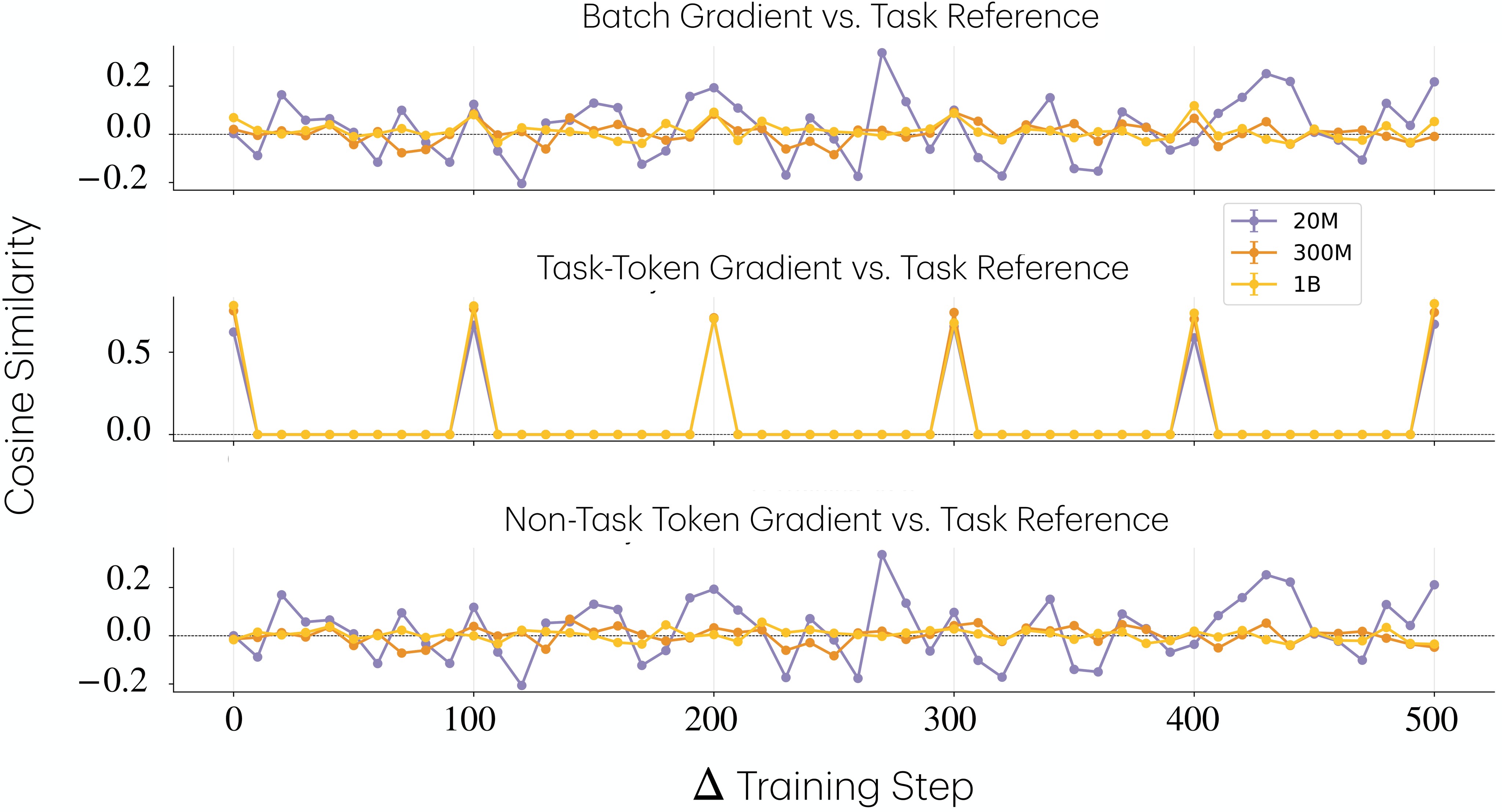
For representation analysis, the comparison task is localized to a global token-order feature using distributed alignment search. The modular-addition task is analyzed through Fourier modes in the residual stream. For gradient analysis, the authors localize task-relevant MLP neurons, use a task reference direction \(g_r\) from all 10K task instances, and decompose the batch gradient into task-token and non-task-token parts:

g = g_t + g_{\mathit{nt}}.

Experiments And Results

Synthetic Capacity Results

Figure 2 is the main synthetic result for the utility-ranking theorem. It compares empirical retained task features and losses against the analytic top-utility prediction.

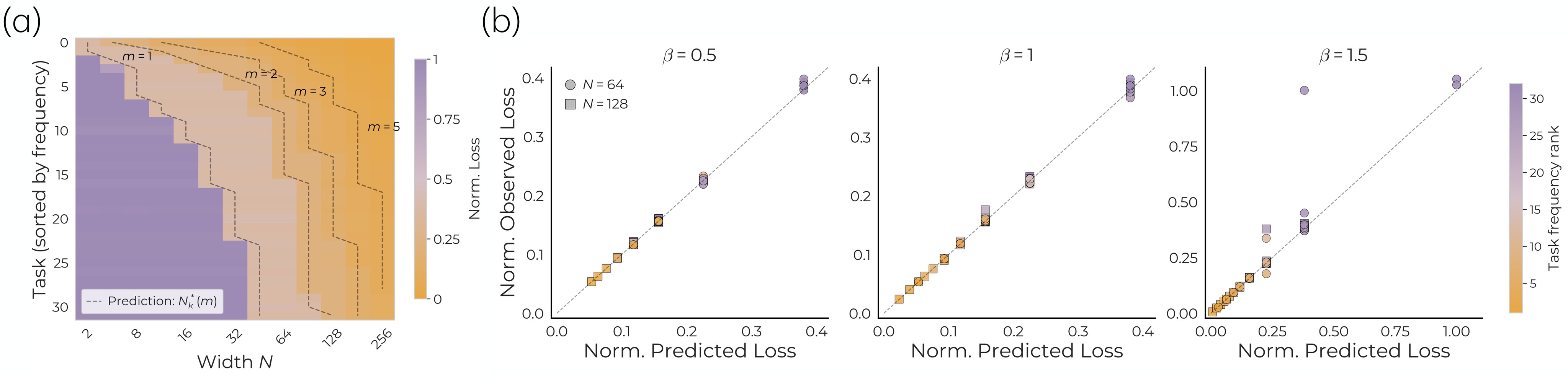
**Figure 2. Feature utility predicts learning order.** The original caption reports a \(K=32\) task mixture with power-law frequencies. Increasing width preferentially improves lower-frequency tasks because it lets the model retain lower-utility features.

The important point is not just that larger models have lower average loss. The phase diagram says which tasks become learnable: the learned region follows the theoretical utility staircase, so width is buying specific low-utility task directions. This directly supports C2.

The long-horizon check in Figure 10 addresses the possible objection that small models simply need more optimization time.

Figure 10. Long-horizon phase diagram. — **Figure 10. Persistence of the multi-rank phase diagram at 1M steps.** The appendix extends selected widths from 100K to 1M steps. Tasks that fit the width budget drop near zero by the standard horizon and stay there; above-capacity tasks remain near the baseline instead of slowly closing the gap.

Synthetic Interference And Retention

Figure 3 tests the residual-control claim: rare-task signal appears only after enough common-task residual has been explained.

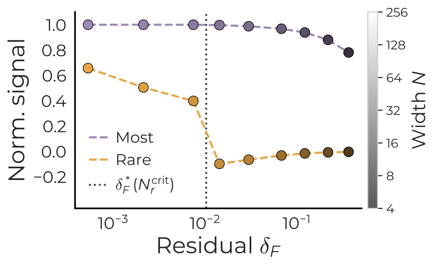
**Figure 3. Residual controls rare-task learning.** The figure plots frequent-task and rare-task representation signal versus width and frequent-task residual \(\delta_{\mathcal{F}}\). Rare-task signal stays near random when common-task residual remains high, then rises once width reduces that residual past the predicted threshold.

Figure 4 isolates rare-task retention by matching long-run frequency while changing the gap \(G\) between rare-task observations.

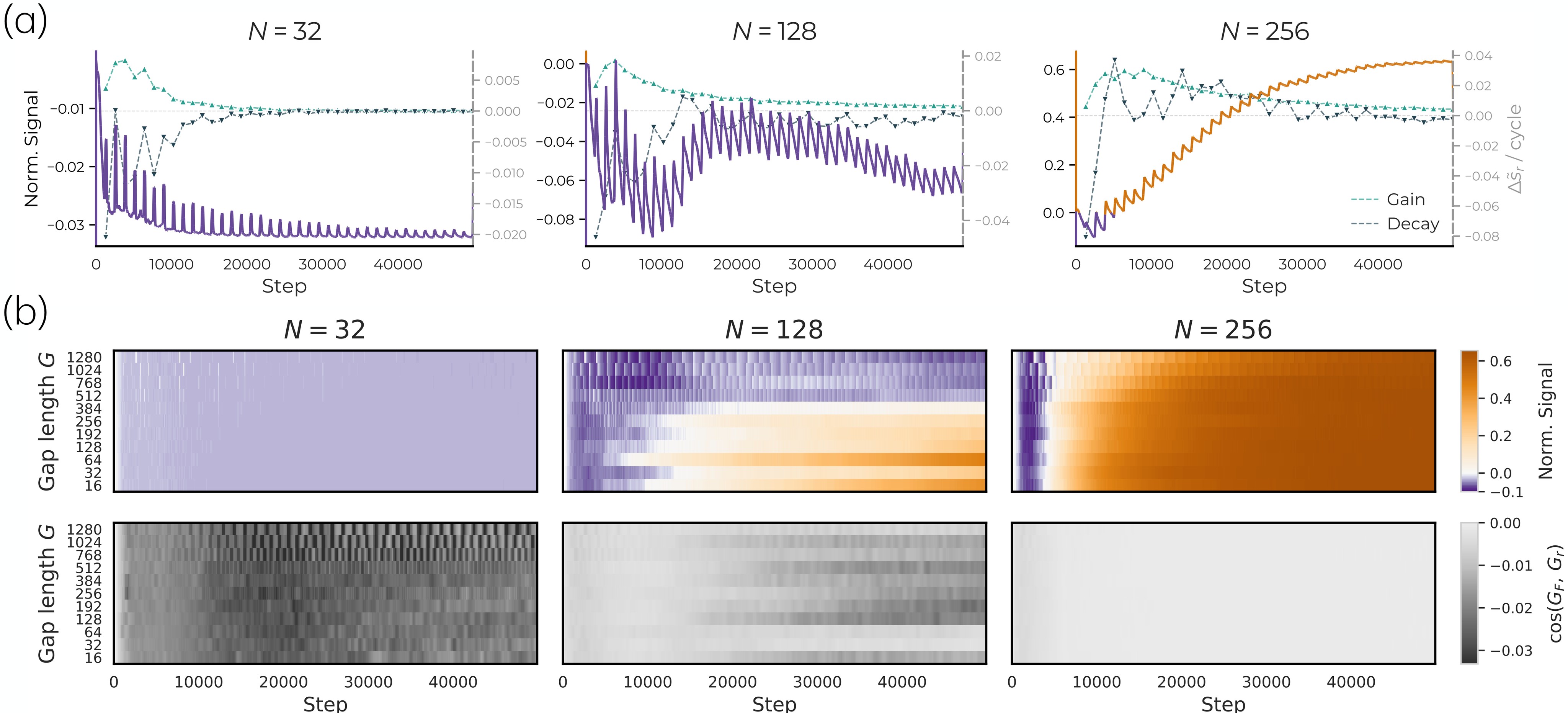
**Figure 4. Rare-task retention by larger models.** Small models briefly encode the rare task after an injection batch, then frequent-task updates erase that signal before the next rare observation. Larger models retain more of the rare-task signal between injections and accumulate it over training.

Together, Figure 3 and Figure 4 give the paper's strongest mechanism evidence. The rare task is not impossible for the architecture in isolation; it loses the competition inside the mixed training stream until width reduces common-task pressure.

OLMo Behavioral Evidence

The OLMo validation asks whether the controlled synthetic pattern survives in a language-model pretraining pipeline. Figure 5 shows that larger OLMo models learn lower-frequency injected comparison and modular-addition tasks that smaller models do not.

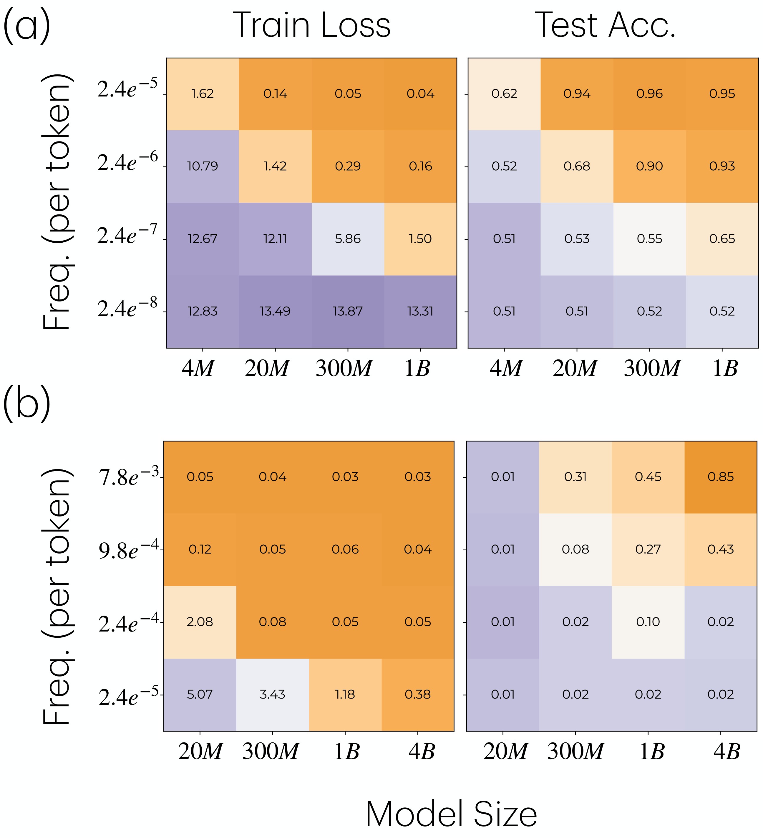
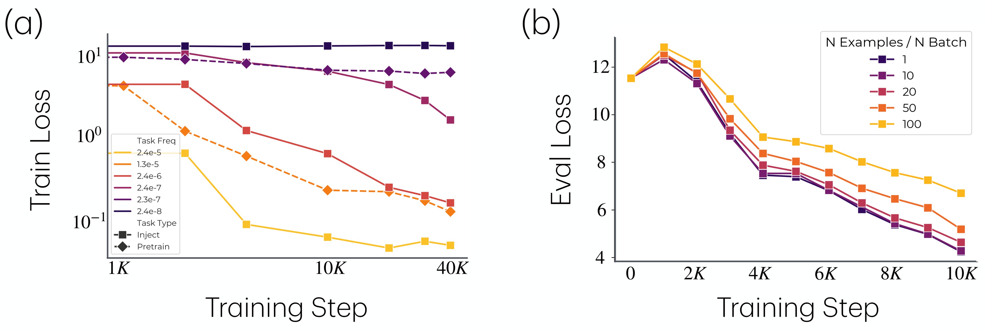
Figure 5. OLMo phase diagrams. — **Figure 5. Larger OLMo models learn rare tasks; smaller models do not.** The figure visualizes training loss and test accuracy for comparison and modular addition. Orange corresponds to lower loss or higher accuracy. The paper emphasizes that larger models are not merely memorizing training instances; the larger models also generalize on held-out task instances.

Figure 6 adds two behavioral checks: tasks are learned in frequency order, and larger gaps between matched-frequency injections hurt learning.

Figure 6. OLMo behavioral evidence. — **Figure 6. Behavioral evidence in OLMo.** Panel (a) injects the comparison task at different frequencies and compares it with reference arithmetic tasks from pretraining. Panel (b) keeps total frequency matched but injects larger batches less often; larger injection gaps degrade task loss, supporting the retention mechanism.

The limitation is that these are deliberately injected tasks, not a direct census of naturally occurring tasks in web data. That makes frequency measurable and the mechanism testable, but it also narrows the ecological scope of C4.

OLMo Representation Evidence

Figure 7 asks whether the larger models actually encode the task-relevant structures.

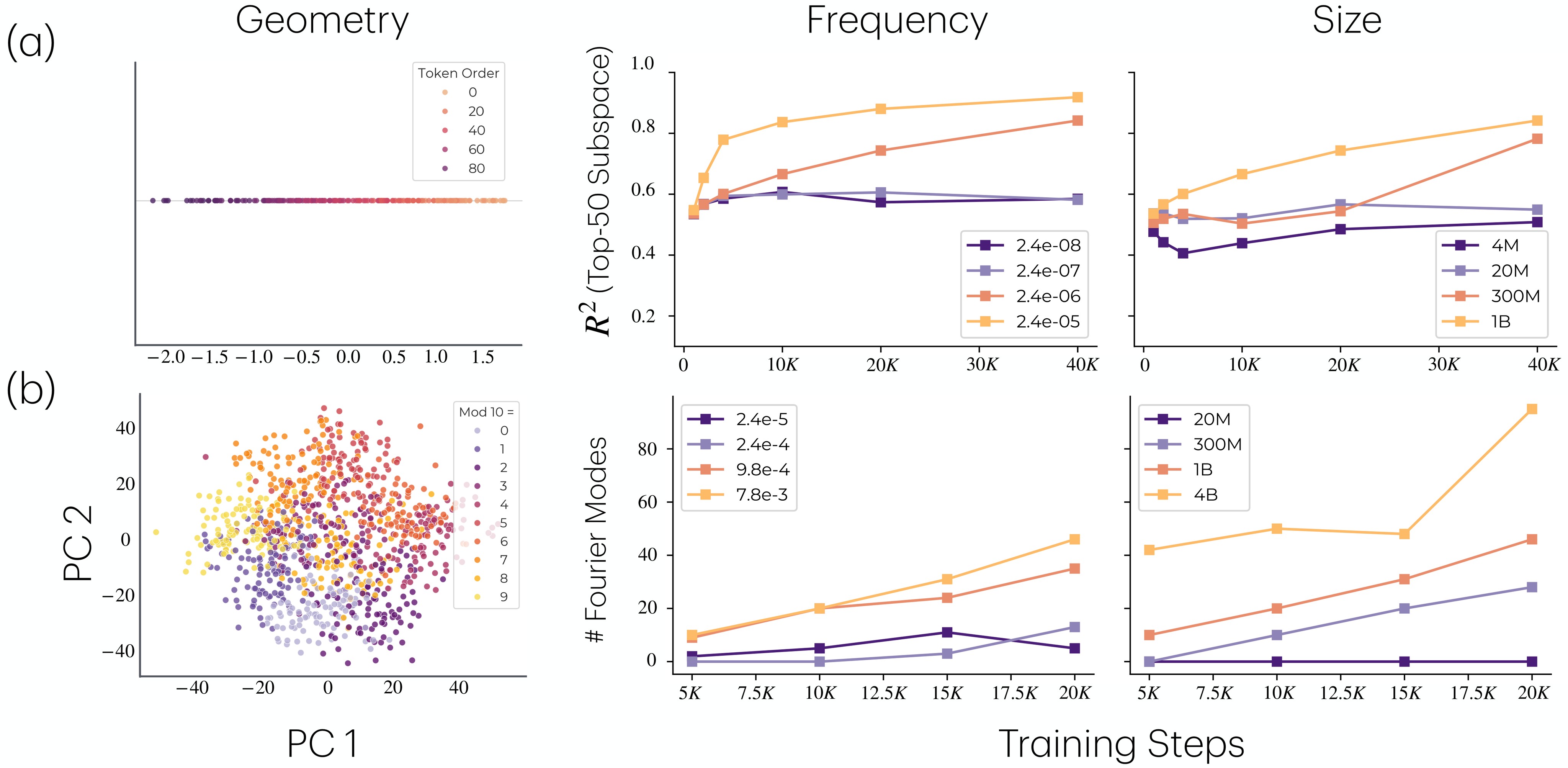
Figure 7. OLMo representational evidence. — **Figure 7. Representational evidence.** For \(T_{\mathrm{CMP}}\), the relevant feature is a global token-order direction. For \(T_{\mathrm{ADD}}\), the relevant features are Fourier modes. The paper reports that larger models and higher task frequencies produce these features faster and more strongly, and that feature presence correlates with high test accuracy.

This matters because the behavioral loss curves could otherwise be read as memorization alone. The representation analysis supports the paper's claim that retained rare-task observations can consolidate into abstract task features.

OLMo Gradient Evidence

The gradient analysis uses localized first-layer MLP neurons and the comparison task. Figure 8 shows that larger models retain more task information after periodic injections.

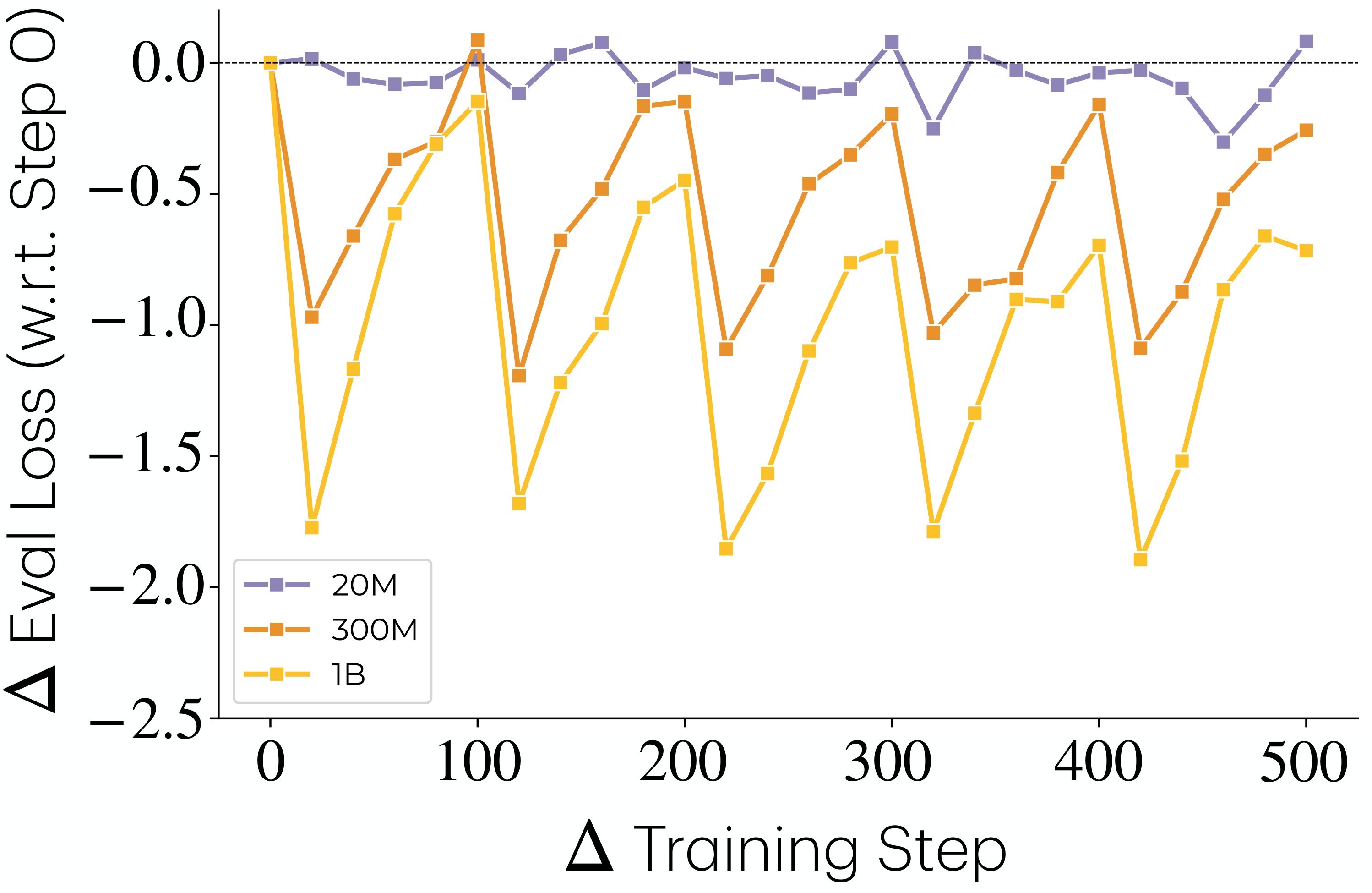
Figure 8. OLMo rare-task retention. — **Figure 8. Rare-task retention in OLMo.** The figure measures task evaluation loss drop when injecting task instances every 100 batches. Larger models retain the injected-task information better.

Figure 9 directly decomposes gradient alignment with the task reference direction \(g_r\).

Figure 9. OLMo gradient interference. — **Figure 9. Gradient interference.** The top panel measures full-batch gradient alignment with \(g_r\); the middle panel isolates task-token gradient; the bottom panel isolates non-task-token gradient. The paper reports that the 1B model has injection-step full-batch similarity \(0.08 +/- 0.02\), the 300M model has \(0.04 +/- 0.04\), and the 20M model oscillates. More importantly, non-task gradient similarity is \(0.10 +/- 0.09\) for the 20M model but \(7.58\times10^{-5} +/- 0.02\) for the 1B model, suggesting much less interference on the localized task neurons.

Data Scaling, Language Modeling Loss, And Compute

Figure 11 compares injected-task loss against general language-modeling loss.

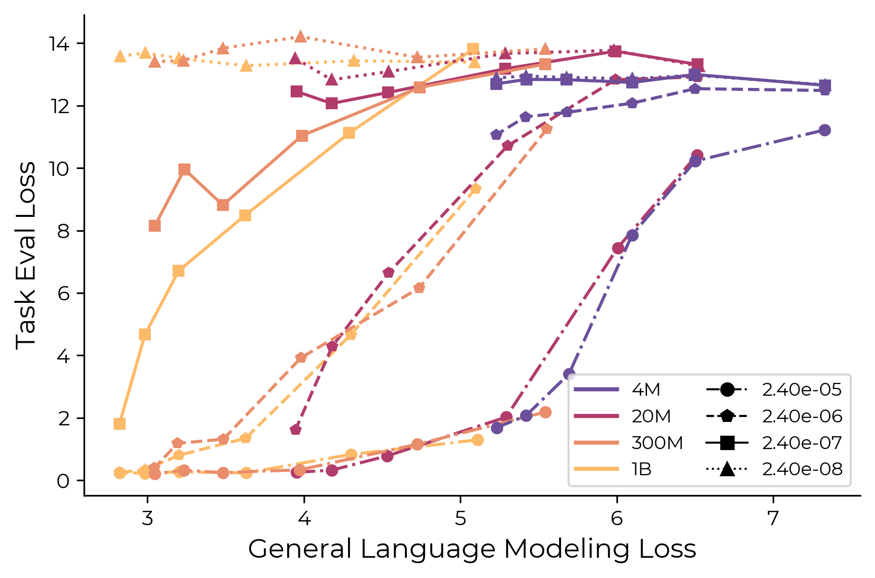
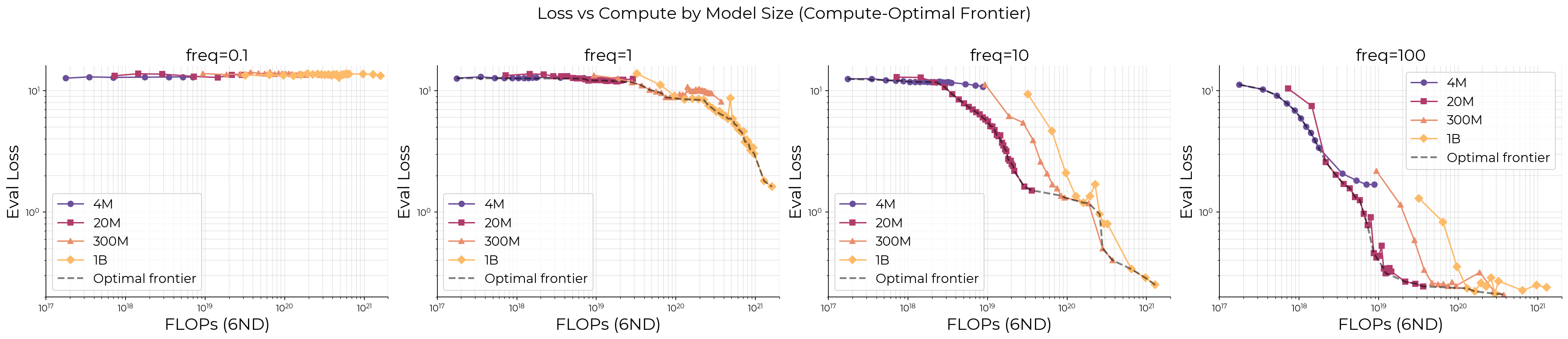
Figure 11. Task loss versus language-modeling loss. — **Figure 11. Task loss versus general language-modeling loss.** For higher injected-task frequencies, all model sizes roughly follow the same trajectory. At the lower frequency \(2.4\times10^{-7}\), larger models achieve lower task loss at the same C4 validation loss, while smaller models plateau.

Figure 12 compares the comparison task against estimated compute.

**Figure 12. Compute-optimal comparison.** For the comparison task at one task instance per batch, the larger models reach lower task loss at the same estimated compute budget. This supports the practical claim that rare-task learning can show different dynamics from ordinary language-modeling improvement.

Practical Takeaways

The most reusable idea is the utility lens: in mixed training, a feature's effective priority is not just "is this task present?" but roughly "how often is it present times how much signal does this feature explain?"
The paper gives a concrete mechanism for why rare tasks can fail in smaller models even when the model could express the task in isolation: frequent-task gradients erase rare-task updates before they accumulate.
Memorization is framed as a useful intermediate for rare-task generalization. The model must retain traces of sparse observations long enough for them to consolidate into abstract features.
Data-mixture design matters. If a target capability is rare, increasing its frequency or reducing gradient interference may be more efficient than increasing model size blindly.
The strongest evidence is controlled: synthetic orthogonal regression tasks plus injected OLMo tasks. This makes the mechanism readable, but it does not prove that every emergent capability in frontier-scale pretraining follows this mechanism.

The limitations section explicitly says this is not a complete account of scaling. Expressivity and sample efficiency still matter, and the OLMo validation does not cover larger-scale or over-trained language models. The injected tasks are chosen to match frequencies of tasks learned in OLMo pretraining, so extreme frequency regimes and naturally occurring task families remain open follow-up questions.