Beyond 3D VQAs: Injecting 3D Spatial Priors into Vision-Language Models for Enhanced Geometric Reasoning

Source-first digest for checked paper rank 13, rank_id p045.

Routing status: success
PDF extraction: not used

Motivation / Background

The paper attacks a recurring weakness in spatial VLMs: models can score well on 3D visual question-answering datasets while still lacking robust geometric representations. The authors argue that fine-tuning on 3D VQA pairs encourages shortcut learning and dataset memorization, while methods that attach explicit 3D encoders, point clouds, object masks, or BEV features add latency and alignment problems.

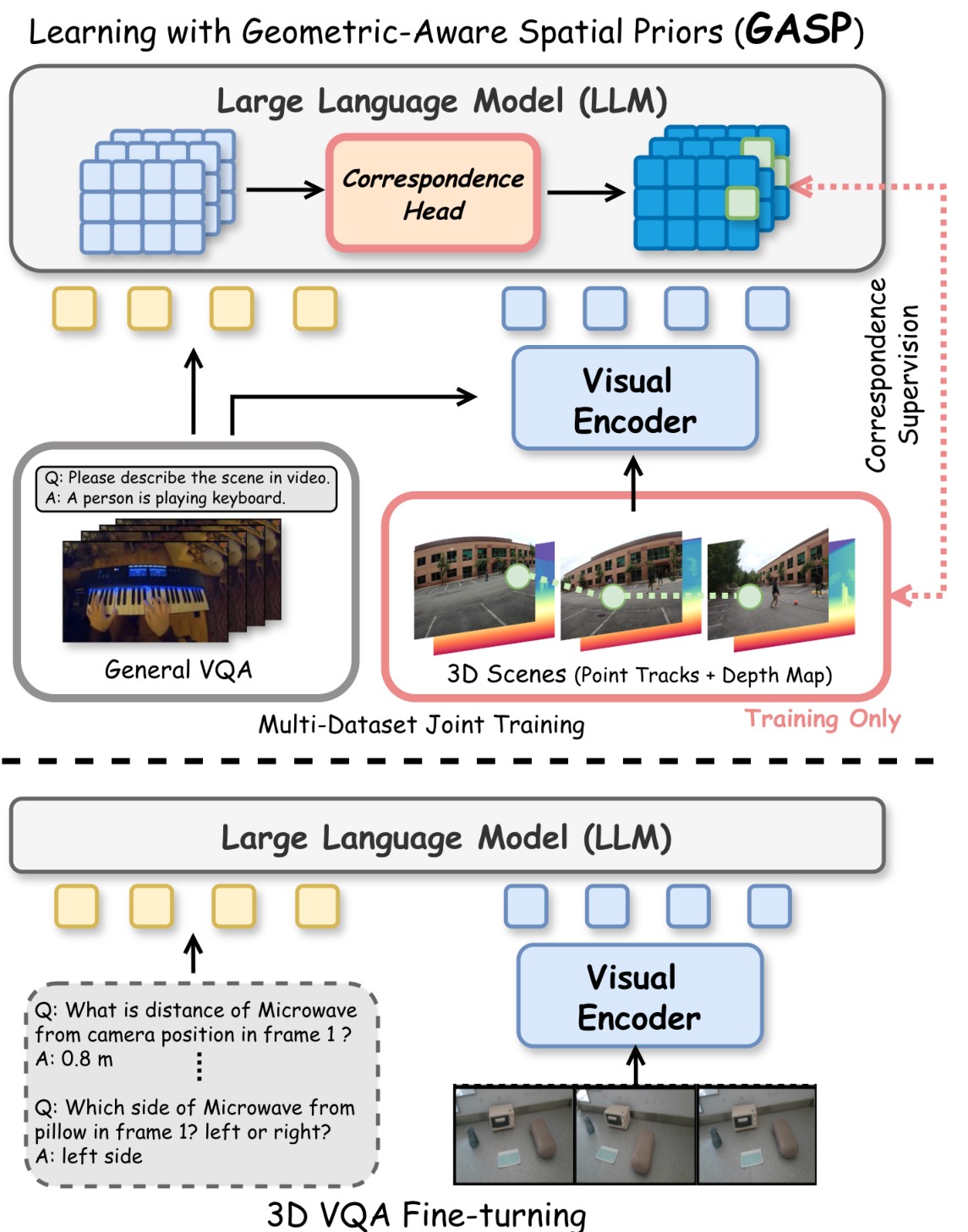
GASP proposes a different training signal. Instead of teaching the model more spatial QA patterns, it teaches the model to preserve visual correspondence across camera movement. The paper's problem framing is summarized in Figure 1: standard spatial VLMs learn from 3D VQA labels, while GASP injects correspondence and depth supervision into the LLM backbone during training and then removes the auxiliary head at inference.

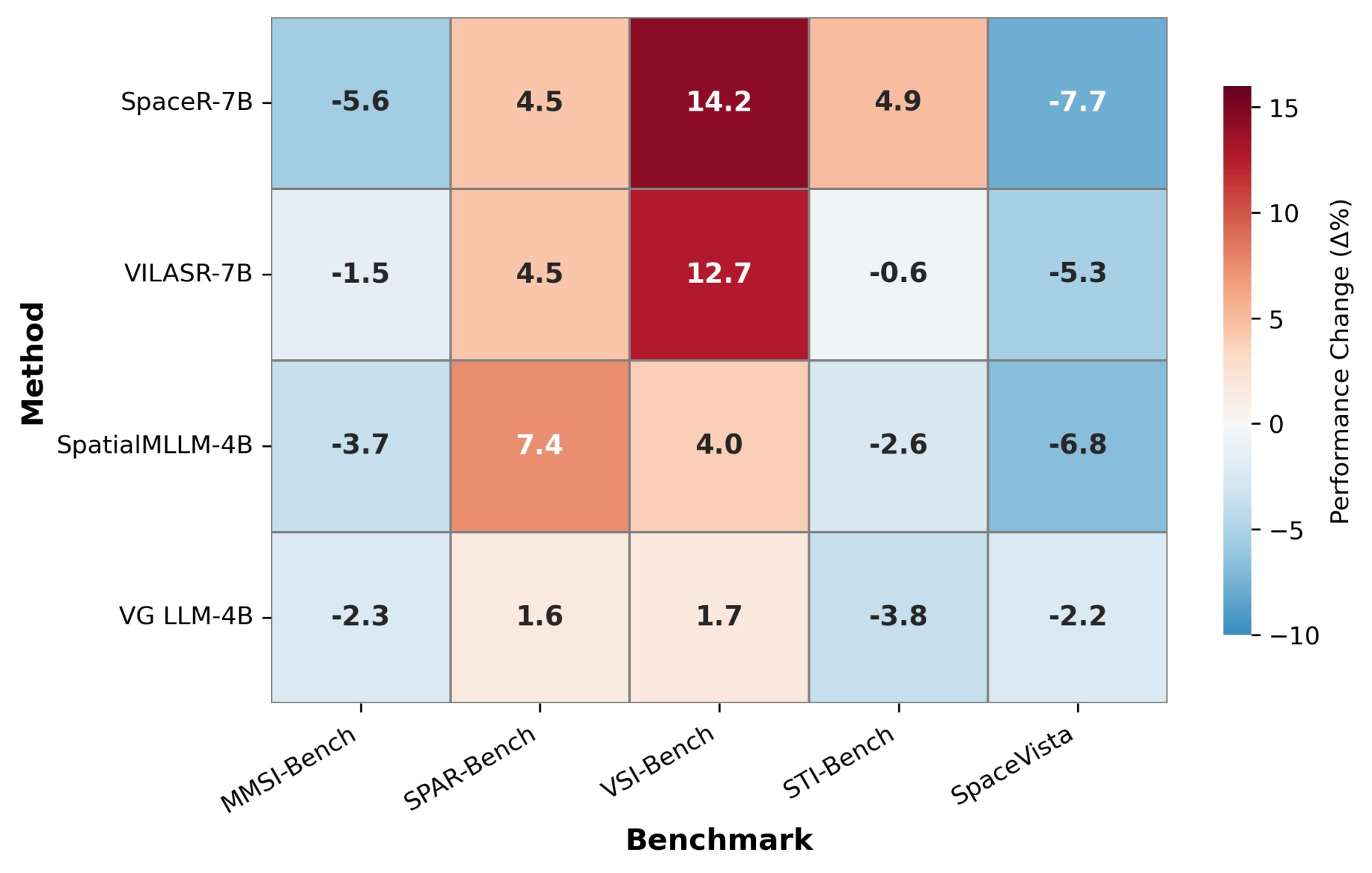
**Figure 1. GASP versus 3D-VQA fine-tuning.** Original caption: Top: GASP learns geometric consistency by injecting the correspondence head into the LLM, supervised by 3D spatial priors. Bottom: standard spatial VLMs rely on fine-tuning with 3D VQA datasets, which often leads to memorizing data-specific biases. GASP requires no 3D prior input and runs as a standard VLM during inference.

The appendix adds concrete evidence that VQA-only supervision can be brittle. Figure 4 shows specialized spatial VLMs improving on VSI-Bench while degrading on out-of-domain spatial benchmarks. Table 5 also shows that adding simple average object and room-size priors to prompts can sharply improve VSI-Bench-style scores, especially for object absolute distance, which supports the paper's concern that some benchmark gains can be shortcut-driven.

**Figure 4. Generalization gap in 3D-VQA fine-tuning.** Original caption: performance changes of specialized spatial VLMs relative to their underlying backbones across five spatial benchmarks. Fine-tuning improves specific datasets such as VSI-Bench but causes degradation on out-of-distribution benchmarks such as MMSI-Bench and SpaceVista, suggesting task-specific overfitting rather than general spatial understanding.

Claims And Evidence

Claim id	Main claim	Support	Evidence anchors
C1	3D-VQA fine-tuning alone can overfit benchmark-specific spatial shortcuts rather than learning general spatial reasoning.	4	problem framing, bias hack, 3D-VQA generalization
C2	Direct geometric supervision on internal visual representations substantially improves VLM correspondence behavior.	5	method overview, correspondence and depth losses, internal analysis
C3	The correspondence head can act as a training-time scaffold: the inference-time model remains a standard RGB VLM without 3D inputs.	3	method overview, training details, gradient mechanism
C4	GASP's geometric objective improves downstream spatial reasoning more than controlled SFT or DL3DV data exposed as VQA.	5	spatial results, controlled baselines
C5	Geometric training does not catastrophically damage general video/VQA ability, but it does introduce a small task trade-off.	4	general multimodal benchmarks, CV-Bench, limitations
C6	The best downstream configuration is not simply the one with maximum internal PCK; LoRA rank and all-layer injection matter.	4	ablation, method details

Scores are support-from-paper scores, not independent reproduction scores. Claims about generality are capped where evidence is limited to the tested 7B backbones, selected spatial benchmarks, and pseudo ground-truth geometry.

Core Technical Idea

The paper starts from the visual self-attention block inside a VLM. Visual tokens \(V\) and language tokens \(L\) are concatenated before the LLM backbone:

X = \mathrm{Concat}(V,L).

For each transformer layer, the attention matrix decomposes into visual-visual, visual-language, language-visual, and language-language blocks:

S = QK^T = \begin{pmatrix} Q_V K_V^T & Q_V K_L^T \\ Q_L K_V^T & Q_L K_L^T \end{pmatrix}.

GASP focuses on \(Q_V K_V^T\), because this block directly exposes whether visual tokens can match corresponding scene points across frames. The paper's core hypothesis is that high-level spatial reasoning improves when the model's internal visual self-attention is forced to become geometrically consistent. Figure 2 is the compact view of how this auxiliary supervision enters training and then disappears at inference.

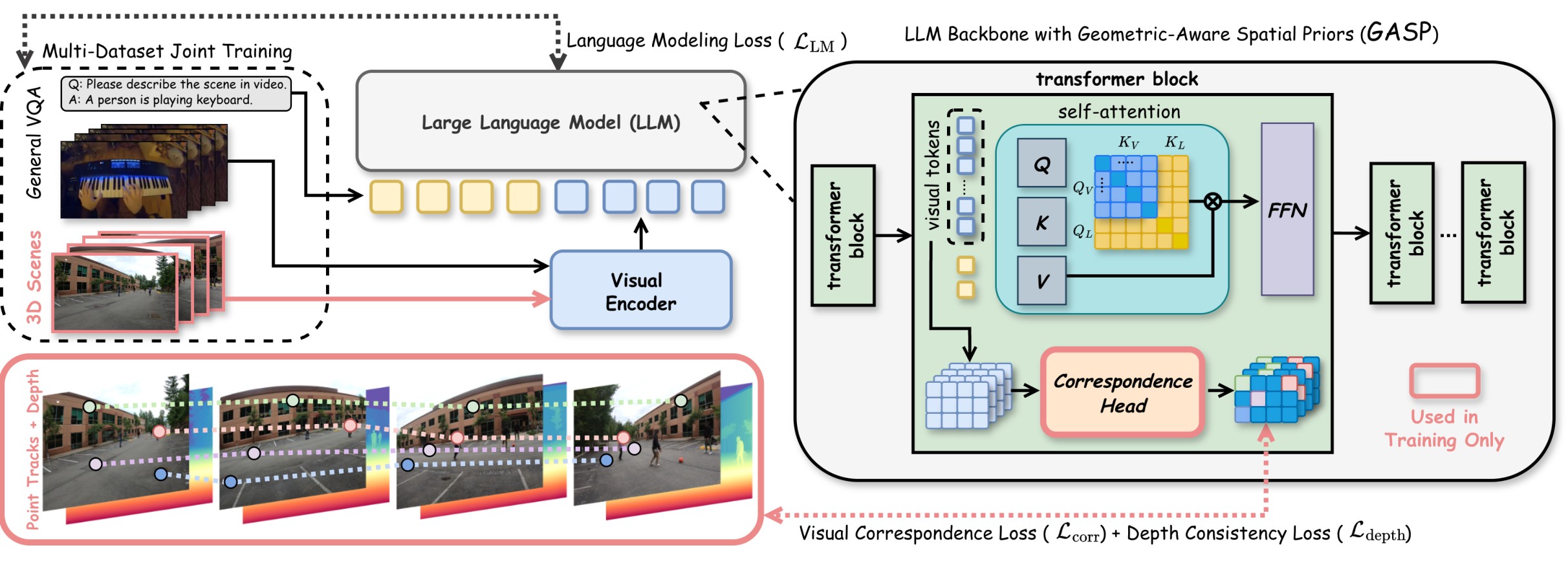
**Figure 2. GASP training framework.** Original caption: GASP inserts a small correspondence head into intermediate LLM layers. During training, the head receives visual correspondence and depth-consistency supervision from ground-truth point tracks and depth maps. At inference, the head is discarded and the model processes VQA inputs as a standard VLM without auxiliary 3D input.

The method attaches a lightweight correspondence head \(\mathcal{H}_c\) to transformer-layer visual tokens:

\mathbf{E} = \mathcal{H}_c(V^{(l)}),

where \(\mathbf{E}\) is a set of correspondence-aware embeddings. The head is initialized from the layer's query projection matrix via SVD, which is meant to make the auxiliary head less disruptive to the pretrained model. The source text describes the head as a 2-layer MLP; the supplement gives the concrete hidden dimensions as \(d_h=3584\) for Qwen2.5-VL-7B and \(d_h=4096\) for LLaVA-NeXT-Video-7B.

Correspondence Loss

For an anchor point in frame \(a\), the matching point in frame \(b\) is positive and all other candidate points in frame \(b\) are negatives. GASP trains correspondence embeddings with InfoNCE:

\mathcal{L}_{i} = -\log \frac{ \exp(\langle \mathbf{e}_i^a,\mathbf{e}_i^b\rangle/\tau) }{ \exp(\langle \mathbf{e}_i^a,\mathbf{e}_i^b\rangle/\tau) + \sum_{k \neq i}\exp(\langle \mathbf{e}_i^a,\mathbf{e}_k^b\rangle/\tau) }.

This is the object-constancy part of the method: matched 3D points should remain close in embedding space even when their 2D image positions change.

Depth Consistency

The contrastive score also defines a soft matching distribution:

\mathbf{A}_{ij} = \frac{\exp(\langle \mathbf{e}_i^a,\mathbf{e}_j^b\rangle/\tau)} {\sum_{k=1}^{N_{\mathrm{cand}}}\exp(\langle \mathbf{e}_i^a,\mathbf{e}_k^b\rangle/\tau)}.

GASP computes the expected target-frame depth

\hat{d}_i^b = \sum_{j=1}^{N_{\mathrm{cand}}} \mathbf{A}_{ij} d_j^b,

and penalizes mismatch with the ground-truth target depth:

\mathcal{L}_{\mathrm{depth}} = \frac{1}{N_{\mathrm{valid}}} \sum_{i \in \mathrm{valid}} \frac{|d_i^b-\hat{d}_i^b|} {d_i^b+\hat{d}_i^b+\epsilon}.

The final training objective is:

\mathcal{L}_{\mathrm{total}} = \mathcal{L}_{\mathrm{LM}} + \lambda_c \mathcal{L}_{\mathrm{corr}} + \lambda_d \mathcal{L}_{\mathrm{depth}}.

The depth term is not trained as a depth estimator. It acts as a discriminative regularizer so visually similar patches at incompatible depths do not become easy false matches.

Method Details

Training Data And Optimization

The training recipe uses DL3DV-derived video scenes and LLaVA-Video-178K. The authors generate point correspondences from multi-view video, depth maps, camera intrinsics, and camera extrinsics following a VGGT-style annotation recipe. For each scene they sample an anchor frame and 8 to 24 nearby frames within a temporal radius \(R=48\), producing about 1.75M sequences with coarse \(8 \times 8\) and fine \(24 \times 24\) point grids. LLaVA-Video-178K is interleaved to preserve general video-language ability.

The reported optimization setup uses Qwen2.5-VL-7B and LLaVA-NeXT-Video-7B. The main experiment section says the model is fine-tuned with LoRA rank 512, AdamW, peak learning rate \(10^{-4}\), gradient clipping 1.0, bfloat16, and gradient checkpointing for roughly 10 hours on 32 H200 GPUs. The supplementary implementation details refine the rank choice: rank 512 for LLaVA-NeXT-Video-7B and rank 128 for Qwen2.5-VL-7B, applied to \(W_Q,W_K,W_V,W_O\). This matches the ablation result in Table 4, where those ranks maximize downstream performance for their respective backbones.

Why The Head Can Be Removed

The paper's mechanism argument is that the auxiliary head is not the final representation used at inference. The geometric losses backpropagate through the head into the transformer's query/key/value projectors. In simplified form:

\frac{\partial \mathcal{L}_{\mathrm{corr}}}{\partial \theta^{(l)}} = \frac{\partial \mathcal{L}_{\mathrm{corr}}}{\partial E} \frac{\partial \mathcal{H}_c(V^{(l)})}{\partial V^{(l)}} \frac{\partial V^{(l)}}{\partial \theta^{(l)}}.

The paper argues that this reshapes \(W_Q^T W_K\), making standard attention assign higher similarity to geometrically corresponding, depth-consistent tokens. That is why the authors can discard \(\mathcal{H}_c\) after training while retaining an RGB-only VLM. The claim is mechanistically plausible and supported by downstream results, but it is not independently verified by a runtime ablation of the removed head.

Experiments And Results

Internal Correspondence Analysis

Figure 3 is the paper's direct evidence that GASP changes internal geometry rather than only tuning final VQA answers. The evaluation uses 200 held-out DL3DV sequences, dense \(8 \times 8\) point correspondences across 8 frames, and PCK with a 2-patch threshold. It evaluates layer-wise matching, confidence-accuracy correlation, and robustness as temporal frame gap increases.

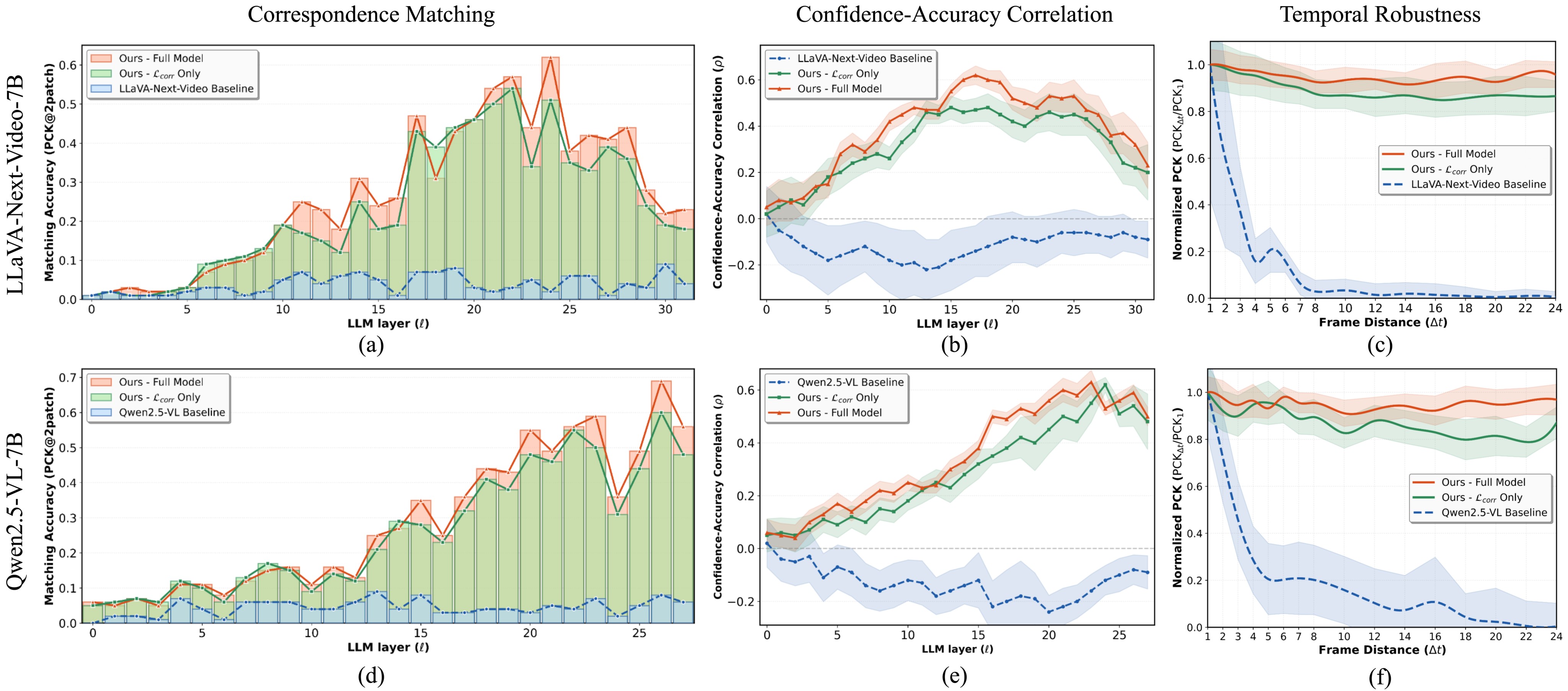
**Figure 3. Visual correspondence learning.** Original caption: analysis on LLaVA-NeXT-Video-7B and Qwen2.5-VL-7B comparing layer-wise PCK, confidence-accuracy correlation \(\rho\), and temporal robustness for GASP against baselines. Shaded regions indicate standard deviation across 200 test sequences.

The source text reports that baselines have near-zero PCK, while GASP improves matching across middle-to-deep layers. Baseline confidence is negatively correlated with correctness, around \(\rho \approx -0.22\), meaning high-confidence matches are often wrong. GASP full reaches about \(\rho \approx +0.62\). Temporal robustness is also stronger: baselines retain less than 5% of their shortest-gap performance beyond an 8-frame gap, while the full model maintains over 85% at 24-frame distances.

Spatial Reasoning Benchmarks

The main controlled comparison is against two baselines: continued SFT on LLaVA-Video-178K and a fairness baseline that reformulates DL3DV correspondence data as VQA. This matters because the strongest question is whether gains come from geometry as an objective or simply from extra exposure to DL3DV data.

Backbone / method	All-Angles camera pose	VSI object count	VSI relative direction	BLINK multi-view
LLaVA-NeXT-Video-7B, LLaVA-Video SFT baseline	22.7	23.5	32.4	42.1
LLaVA + DL3DV as VQA	19.8	21.4	31.8	42.5
LLaVA + GASP correspondence only	34.7	39.8	30.5	44.4
LLaVA + GASP full	40.9	52.5	41.2	57.1
LLaVA full delta over baseline	+18.2	+29.0	+8.8	+15.0
Qwen2.5-VL-7B, LLaVA-Video SFT baseline	34.1	33.8	34.3	41.5
Qwen + DL3DV as VQA	31.5	33.2	34.3	42.0
Qwen + GASP correspondence only	50.0	39.6	36.7	54.9
Qwen + GASP full	52.8	41.6	40.6	53.4
Qwen full delta over baseline	+18.7	+7.8	+6.3	+11.9

Table 1. Condensed main spatial benchmark results. The original table also reports manipulation, route planning, appearance order, spatial relation, and relative depth columns, plus broader general-VLM and 3D-spatial-VLM baselines. This condensed view keeps the most claim-relevant controlled rows and the tasks explicitly highlighted by the authors.

The results support two separate conclusions. First, geometry-objective training beats the controlled SFT baseline on most displayed spatial tasks. Second, the DL3DV-as-VQA baseline can be worse than ordinary SFT, so the improvement is not simply from exposing the model to the same scene content.

General Multimodal Benchmarks

Backbone / method	Video-MME no subtitles	Video-MME with subtitles	TempCompass MC	NextQA
LLaVA-NeXT-Video-7B baseline	40.8	40.3	50.1	59.4
LLaVA + GASP correspondence	42.3	41.6	53.7	62.8
LLaVA + GASP full	42.8	41.9	53.8	61.6
Qwen2.5-VL-7B baseline	60.6	59.3	68.4	76.6
Qwen + GASP correspondence	62.6	61.2	71.5	78.4
Qwen + GASP full	63.2	61.6	70.3	74.7

Table 2. Generic multimodal benchmark comparison. GASP improves Video-MME and TempCompass for both backbones. For Qwen2.5-VL-7B, the full model drops on NextQA from 76.6 to 74.7, while correspondence-only reaches 78.4. This supports the paper's own caveat: geometric specialization helps spatial/temporal consistency but can trade off with action-centric QA.

Method	CV-Bench overall	2D count	2D relation	3D depth	3D distance
Qwen2.5-VL-7B-Instruct	76.6	63.7	87.7	85.5	72.7
Qwen + GASP correspondence	79.4	68.0	88.1	86.6	78.6
Qwen + GASP full	79.8	68.2	88.3	87.3	79.2
Qwen2.5-VL-32B	79.7	68.9	80.8	86.5	85.8
LLaVA-OneVision-72B	79.7	70.2	89.2	82.5	79.0

Table 3. CV-Bench comparison. The paper highlights that Qwen2.5-VL-7B with GASP reaches 79.8 overall, slightly above several much larger references in this table, while not leading every subcategory.

Ablations

Setting	Avg PCK	All-Angles	VSI-Bench	BLINK
LLaVA rank 512	26.2	38.1	37.1	51.0
LLaVA rank 1024	28.6	37.2	34.8	48.7
Qwen rank 128	26.7	43.4	36.9	74.3
Qwen rank 1024	32.5	38.9	33.2	73.8
LLaVA layer 25-32	25.8	39.1	36.5	49.3
LLaVA all layers 1-32	26.2	38.1	37.1	51.0
Qwen layer 22-28	25.2	42.7	37.4	72.8
Qwen all layers 1-28	26.7	43.4	36.9	74.3

Table 4. Ablation summary. Higher internal PCK is not automatically the best downstream setting. The paper interprets this as a capacity trade-off: very high LoRA rank may fit geometric priors more strongly while damaging language or broader reasoning capability. All-layer supervision is generally best or near-best, which supports the hierarchical-geometric-supervision argument.

VSI task	Baseline 7B	7B + average prior	Baseline 72B	72B + average prior	VLM-3R
Object size estimation	0.47	0.64 (+0.17)	0.57	0.65 (+0.08)	0.69
Room size estimation	0.24	0.38 (+0.14)	0.36	0.46 (+0.10)	0.67
Object absolute distance	0.14	0.61 (+0.47)	0.23	0.57 (+0.34)	0.49

Table 5. VSI-Bench bias hack. The textual average-prior prompt sharply improves distance and size estimates, showing that some spatial benchmark scores can be boosted by dataset-level priors rather than visual 3D reasoning.

Practical Takeaways

The most reusable idea is to train geometry into the VLM's internal visual attention, not to add a permanent 3D encoder or simply fine-tune on more 3D VQA labels.
GASP is a source-efficient recipe: passive RGB video plus camera/depth-derived correspondences become supervision for object permanence and depth-aware matching.
Internal evaluation matters. The PCK, confidence-calibration, and temporal-robustness analyses in Figure 3 are more diagnostic than final VQA accuracy alone.
The strongest downstream evidence is controlled: same base backbones, ordinary video SFT, DL3DV-as-VQA, correspondence-only GASP, and full correspondence-plus-depth GASP.
The weak point is generality beyond the tested scope. Results are on two 7B backbones and selected spatial/video benchmarks, using pseudo ground-truth geometry from existing reconstruction pipelines.
The paper itself acknowledges two important caveats: reliance on pseudo ground-truth depth, and a modest trade-off on action-centric tasks such as NextQA. GASP looks best suited for robotics, multi-view perception, and spatial geometry workloads where geometry is primary.

The conclusion states that GASP corrects near-zero internal correspondence accuracy to over 70% and improves downstream spatial benchmarks, while noting limitations from pseudo ground-truth depth and small action-centric trade-offs. A natural follow-up would be to test larger backbones, more diverse camera domains, and robotics tasks where correspondence quality directly affects embodied decisions.