Source-first digest for checked paper rank 49, rank_id p055.
- Table recovery source:
latex_flattened/main.flattened.tex, used only because the main numeric result tables are empty inpaper.md - Routing status:
success - PDF extraction: not used
Motivation / Background
Time-series anomaly detection is usually evaluated as a numeric labeling problem: identify abnormal points or intervals, then report precision, recall, or F1. The paper argues that this is too thin for operational use because practitioners often need to know why a region is abnormal, whether the predicted interval is temporally aligned, and whether the explanation is grounded in the visible trend rather than a generic alarm.
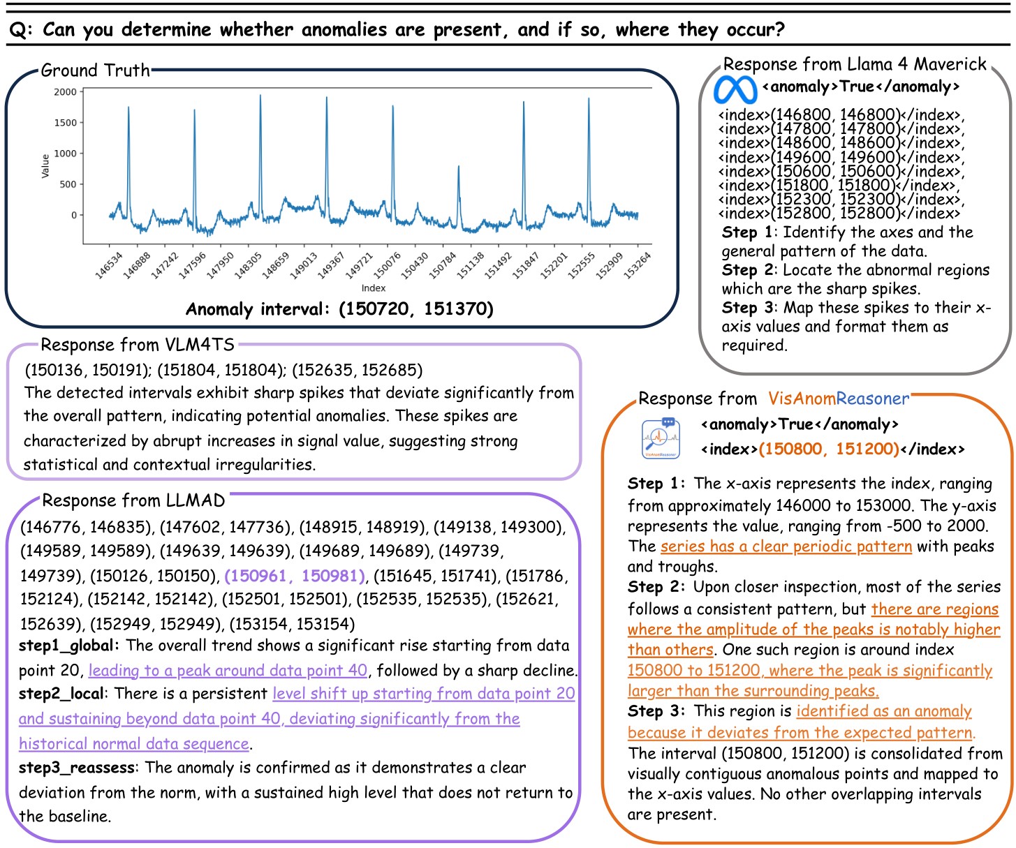
The paper's response is to treat anomaly detection as plot-grounded vision-language reasoning. A model receives a rendered univariate time-series plot and optional context, then outputs structured anomaly tags, interval indices, and a step-by-step explanation. Figure 1 shows the intended behavior: VisAnomReasoner localizes the anomalous interval and ties the decision to observable periodicity and amplitude deviations, while comparison methods overflag spikes or produce generic rationales.
Claims And Evidence
| Claim id | Main claim | Support | Evidence anchors |
|---|---|---|---|
| C1 | Time-series anomaly detection can be reformulated as a plot-grounded vision-language task that jointly predicts anomaly intervals and natural-language reasoning. | 4 | task formulation, dataset construction, qualitative example |
| C2 | VisAnomBench supplies explanation-augmented supervision at meaningful scale by augmenting public anomaly datasets with reward-selected VLM explanations. | 4 | dataset construction, dataset statistics, source composition, multi-model supervision, reward objective |
| C3 | VisAnomReasoner outperforms 15 general VLM, small VLM, foundation-model, specialized-model, and classical-detector baselines on VisAnomBench. | 5 | VisAnomBench results, main benchmark table |
| C4 | The 7B variant generalizes to the separate TSB-AD-U benchmark better than the reported baselines. | 4 | TSB-AD-U results, TSB-AD-U table |
| C5 | Explanation-augmented supervision improves anomaly localization beyond interval-only fine-tuning. | 4 | SFT bar chart, reasoning ablation, explanation preference |
| C6 | A small, parameter-efficient VLM can be competitive with much larger VLMs for this task. | 4 | model and LoRA setup, VisAnomBench results, TSB-AD-U results, efficiency note |
| C7 | The generated explanations are more visually grounded and useful than baseline explanations. | 3 | qualitative example, additional qualitative example, explanation preference, limitations |
Scores are support-from-paper scores, not independent reproduction scores. I cap the explanation-quality and generalization claims where the evidence relies on model-judged explanations, synthetic supervision, one univariate plotting setup, or a fixed subset of TSB-AD-U.
Core Technical Idea
The method keeps the raw time series outside the language context window by rendering it as an image. For a univariate series \(x=\{x_1,\ldots,x_T\}\), ground-truth anomalies are intervals \(\mathcal{A}^\star=\{(s_i^\star,e_i^\star)\}_{i=1}^m\). A VLM receives the plot \(I(x)\) and optional context \(C\), then returns predicted intervals \(A\) and a reasoning trace \(E\):
The structured target contains <anomaly> tags for the anomaly decision, <index> tags for interval localization, and <think> tags for the step-by-step explanation. This makes the paper less about a new time-series detector architecture and more about an instruction-tuned chart-reasoning detector: anomaly detection is supervised as a visual reasoning response.
The benchmark construction is the other core component. Instead of asking humans to write rationales for thousands of time-series windows, the authors generate candidate outputs from four large VLMs, then select the candidate with the best reward. The reward combines interval overlap and explanation quality:
The anomaly score is a length-weighted, range-based F1 over interval overlap. The explanation-quality terms judge visual groundedness, axis awareness, and clarity. In the appendix, the weights are \(\lambda_{\text{ano}}=0.3\), \(\lambda_{\text{vis}}=0.3\), \(\lambda_{\text{axi}}=0.1\), and \(\lambda_{\text{cla}}=0.3\), with Qwen2.5-VL-72B used as the explanation-quality judge.
Method Details
Benchmark Construction
VisAnomBench draws windows from four public univariate anomaly-detection sources: KPI, GutenTAG, UCR-EGI, and UCR-TSAD. The preprocessing keeps windows with anomaly ratio at most 10 percent, centers the anomaly interval between 30 percent and 70 percent of the segment, and requires segment length of at least 200 points. Candidate examples are filtered when multiple VLMs fail to identify the anomaly or consistently disagree with the provided interval, which is meant to remove label-noise cases rather than visually difficult ones.
Table 1 gives the source composition of the benchmark; Table 2 shows that the selected supervision targets come from all four generator models rather than a single teacher.
| Benchmark | TS count | Domains | Avg length | Anomaly ratio | Explanation count | Avg explanation words |
|---|---|---|---|---|---|---|
| KPI | 160 | 1 | 1,777 | 4.3% | 640 | 170 |
| GutenTAG | 810 | 10 | 5,000 | 2.2% | 3,240 | 114 |
| UCR-EGI | 2,097 | 5 | 8,268 | 5.8% | 8,388 | 112 |
| UCR-TSAD | 249 | 8 | 2,755 | 6.9% | 996 | 112 |
Table 1. VisAnomBench source statistics. The table supports C2 by showing that the benchmark combines multiple public anomaly sources with explanation targets. The paper also reports 2,576 training series and 740 held-out test series after filtering.
| Generator selected as supervision source | Grok-4-Fast | LLaMA-4-Maverick | Gemma-3-27B-IT | Qwen2.5-VL-32B |
|---|---|---|---|---|
| Count | 605 | 1,007 | 549 | 415 |
| Percent | 23.5% | 39.1% | 21.3% | 16.1% |
Table 2. Composition of reward-selected supervision. LLaMA-4-Maverick contributes the largest share, but every generator contributes selected examples. This is relevant because the benchmark is synthetic-supervision-heavy.
Model And Training
VisAnomReasoner fine-tunes Qwen2.5-VL-3B and Qwen2.5-VL-7B into 3B and 7B anomaly-reasoning variants. Training is supervised next-token prediction over the selected structured outputs. The paper uses LoRA with 95,178,752 trainable parameters, reported as 1.13 percent of the backbone, and applies LoRA adapters to the vision encoder and projection modules including q_proj, k_proj, v_proj, o_proj, gate_proj, up_proj, and down_proj.
The practical implication is that the learned detector is still a small VLM prompted on a plot image; it is not a direct numerical sequence model. That is also the main limitation: the model can reason over what the plotted image makes visible, but it may miss or hallucinate details if the rendering hides the relevant deviation.
Metrics
The main VisAnomBench evaluation uses interval-level true positives, false positives, false negatives, precision, recall, F1, and an Overlap score. A predicted interval is a true positive if it overlaps a ground-truth interval; extra intervals that do not overlap any ground truth are false positives.
The Overlap metric measures boundary quality and penalizes overextended predictions:
For TSB-AD-U, the paper reports standard point-wise precision/recall/F1 and affiliation metrics, where affiliation scores are more tolerant of small event-boundary offsets.
Experiments And Results
VisAnomBench
Table 3 is the main quantitative evidence for the paper. VisAnomReasoner 7B has the best precision, recall, and F1; VisAnomReasoner 3B has the best Overlap. The nearest baseline precision and F1 are IForest at 48.92 and 48.30, so the 7B model improves precision by 23.17 percentage points and F1 by 25.64 percentage points. The tradeoff is that this is a benchmark built from the same explanation-supervision pipeline the model is trained on, so it is strong in-domain evidence rather than independent deployment proof.
| Method | Category | TP | FP | FN | Precision | Recall | F1 | Overlap |
|---|---|---|---|---|---|---|---|---|
| Grok-4-Fast (314B) | Large VLM | 242 | 837 | 517 | 22.43 | 31.88 | 26.33 | 3.26 |
| LLaMA-4-Maverick (17B) | Large VLM | 442 | 1,128 | 317 | 28.15 | 58.23 | 37.96 | 12.92 |
| Qwen2.5-VL-7B | Small VLM | 517 | 1,784 | 242 | 22.47 | 68.12 | 33.79 | 14.04 |
| Idefics3-8B | Small VLM | 123 | 2,057 | 636 | 5.64 | 16.21 | 8.37 | 2.25 |
| SmolVLM-7B | Small VLM | 49 | 1,416 | 710 | 3.34 | 6.46 | 4.41 | 1.29 |
| LLaVA-7B | Small VLM | 9 | 523 | 750 | 1.69 | 1.19 | 1.39 | 0.23 |
| TimesFM (200M) | Foundation model | 196 | 543 | 563 | 26.52 | 25.82 | 26.17 | 2.03 |
| Chronos (120M) | Foundation model | 200 | 538 | 559 | 27.10 | 26.35 | 26.72 | 2.27 |
| AnomLLM (GPT-4o) | Specialized large model | 149 | 862 | 610 | 14.74 | 19.63 | 16.84 | 4.04 |
| LLM-TSAD (GPT-4o) | Specialized large model | 477 | 5,621 | 282 | 7.82 | 66.53 | 14.00 | 20.81 |
| LLMAD (GPT-4o) | Specialized large model | 349 | 402 | 410 | 46.47 | 45.98 | 46.23 | 17.31 |
| VLM4TS (GPT-4o) | Specialized large model | 435 | 642 | 324 | 40.39 | 57.31 | 47.39 | 17.94 |
| Sub-PCA | Classical detector | 329 | 411 | 430 | 44.46 | 43.35 | 43.90 | 17.41 |
| Matrix Profile | Classical detector | 290 | 450 | 469 | 39.19 | 38.21 | 38.69 | 8.33 |
| IForest | Classical detector | 362 | 378 | 397 | 48.92 | 47.69 | 48.30 | 20.53 |
| VisAnomReasoner (3B) | Ours | 564 | 240 | 195 | 70.15 | 74.30 | 72.17 | 27.07 |
| VisAnomReasoner (7B) | Ours | 576 | 223 | 183 | 72.09 | 75.88 | 73.94 | 25.35 |
Table 3. Main VisAnomBench anomaly-detection results. Values are percentages except TP/FP/FN counts. This table was recovered from latex_flattened/main.flattened.tex because the corresponding paper.md table block is empty.
The failure mode for many baselines is overflagging. Qwen2.5-VL-7B detects 517 true intervals but produces 1,784 false positives; LLM-TSAD detects 477 true intervals but produces 5,621 false positives. This explains why recall can look respectable while precision and F1 collapse. The Overlap column also shows that detecting many points is not enough: LLM-TSAD's high recall gives only 20.81 Overlap because its intervals are too broad or too numerous.
TSB-AD-U Generalization
Table 4 tests the same model family on TSB-AD-U. VisAnomReasoner 7B is strongest on standard recall and F1 and all three affiliation metrics. Qwen2.5-VL-7B remains a strong baseline in standard precision and F1, but the 7B fine-tuned model improves over it by 9.57 points in standard precision, 12.06 in standard recall, and 13.39 in standard F1. This supports cross-benchmark transfer, though the paper notes all experiments use the fixed univariate TSB-AD-U subset.
| Method | Category | Std Precision | Std Recall | Std F1 | Aff Precision | Aff Recall | Aff F1 |
|---|---|---|---|---|---|---|---|
| Grok-4-Fast (314B) | Large VLM | 27.95 | 15.53 | 16.78 | 32.43 | 33.24 | 32.20 |
| LLaMA-4-Maverick (17B) | Large VLM | 63.35 | 46.49 | 48.89 | 76.07 | 79.18 | 76.75 |
| Qwen2.5-VL-7B | Small VLM | 66.18 | 48.85 | 49.52 | 75.90 | 74.93 | 74.36 |
| Idefics3-8B | Small VLM | 45.12 | 35.11 | 34.64 | 50.83 | 59.02 | 53.03 |
| SmolVLM-7B | Small VLM | 35.07 | 12.48 | 15.80 | 37.57 | 35.84 | 35.75 |
| LLaVA-7B | Small VLM | 14.06 | 0.72 | 1.35 | 14.06 | 8.16 | 10.15 |
| TimesFM (200M) | Foundation model | 32.32 | 43.21 | 32.19 | 71.09 | 57.23 | 60.08 |
| Chronos (120M) | Foundation model | 47.18 | 55.37 | 47.23 | 74.36 | 75.61 | 73.31 |
| AnomLLM (GPT-4o) | Specialized large model | 12.97 | 10.54 | 11.63 | 13.05 | 7.08 | 8.42 |
| LLM-TSAD (GPT-4o) | Specialized large model | 31.74 | 28.40 | 29.98 | 66.69 | 52.76 | 53.69 |
| LLMAD (GPT-4o) | Specialized large model | 32.96 | 37.54 | 22.91 | 67.50 | 73.37 | 64.16 |
| VLM4TS (GPT-4o) | Specialized large model | 29.78 | 40.10 | 19.84 | 72.52 | 51.38 | 54.06 |
| Sub-PCA | Classical detector | 11.80 | 16.82 | 12.28 | 48.22 | 31.71 | 34.99 |
| Matrix Profile | Classical detector | 9.40 | 15.84 | 9.91 | 44.90 | 41.44 | 41.90 |
| IForest | Classical detector | 12.44 | 17.89 | 13.05 | 50.44 | 41.51 | 42.67 |
| VisAnomReasoner (3B) | Ours | 77.93 | 40.46 | 49.59 | 95.05 | 71.69 | 78.36 |
| VisAnomReasoner (7B) | Ours | 75.75 | 60.91 | 62.91 | 95.27 | 81.51 | 85.58 |
Table 4. TSB-AD-U benchmark results. Values are percentages. The 3B model has the highest standard precision, while the 7B model has the strongest overall standard F1 and affiliation scores.
Ablations And Explanation Quality
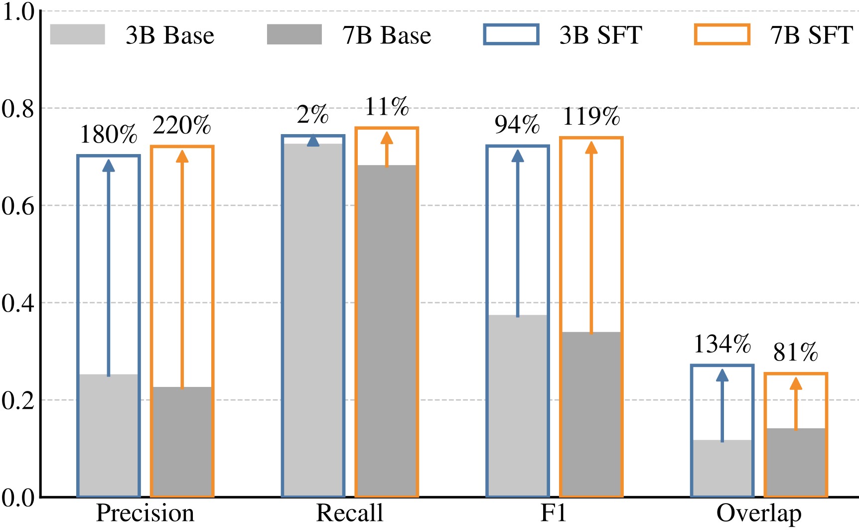
Figure 2 compares base Qwen2.5-VL models against the supervised fine-tuned variants. The visual summary is consistent with the numeric tables: fine-tuning mostly fixes false positives, so precision, F1, and Overlap jump much more than recall.
| Mode | TP | FP | FN | Precision | Recall | F1 |
|---|---|---|---|---|---|---|
| Base | 517 | 1,784 | 242 | 22.47 | 68.12 | 33.79 |
| No reasoning | 516 | 393 | 243 | 56.76 | 67.98 | 61.87 |
| With reasoning | 576 | 223 | 183 | 72.09 | 75.88 | 73.94 |
Table 5. Effect of reasoning supervision. Interval-only fine-tuning reduces false positives but does not recover more true anomalies. Adding reasoning traces improves both TP and FP, raising F1 from 61.87 to 73.94.
The explanation-quality result is less definitive but still informative: GPT-4o chooses the VisAnomReasoner 7B explanation over the base Qwen2.5-VL-7B explanation in 69.6 percent of 740 paired comparisons, chooses the base model in 29.7 percent, and ties in 0.7 percent. The paper also says the authors manually inspected a random subset of selected and rejected candidates during benchmark construction, but it does not report a full human evaluation.
| Training data | TP | FP | FN | Precision | Recall | F1 |
|---|---|---|---|---|---|---|
| SFT with single-model data | 535 | 357 | 224 | 59.98 | 70.49 | 64.81 |
| SFT with VisAnomBench | 576 | 223 | 183 | 72.09 | 75.88 | 73.94 |
Table 6. Effect of multi-model supervision. The full reward-selected VisAnomBench supervision beats training on a single generator's data. This supports the use of multiple generators, but it is not a complete bias audit because only one single-model setting is reported.
Qualitative And Deep TSAD Checks
Figure 3 gives a second qualitative case. It is useful because it shows a different failure mode: LLMAD predicts 147 intervals, LLaMA-4-Maverick gives a plausible but early interval, and VisAnomReasoner keeps the interval closer to the ground truth.
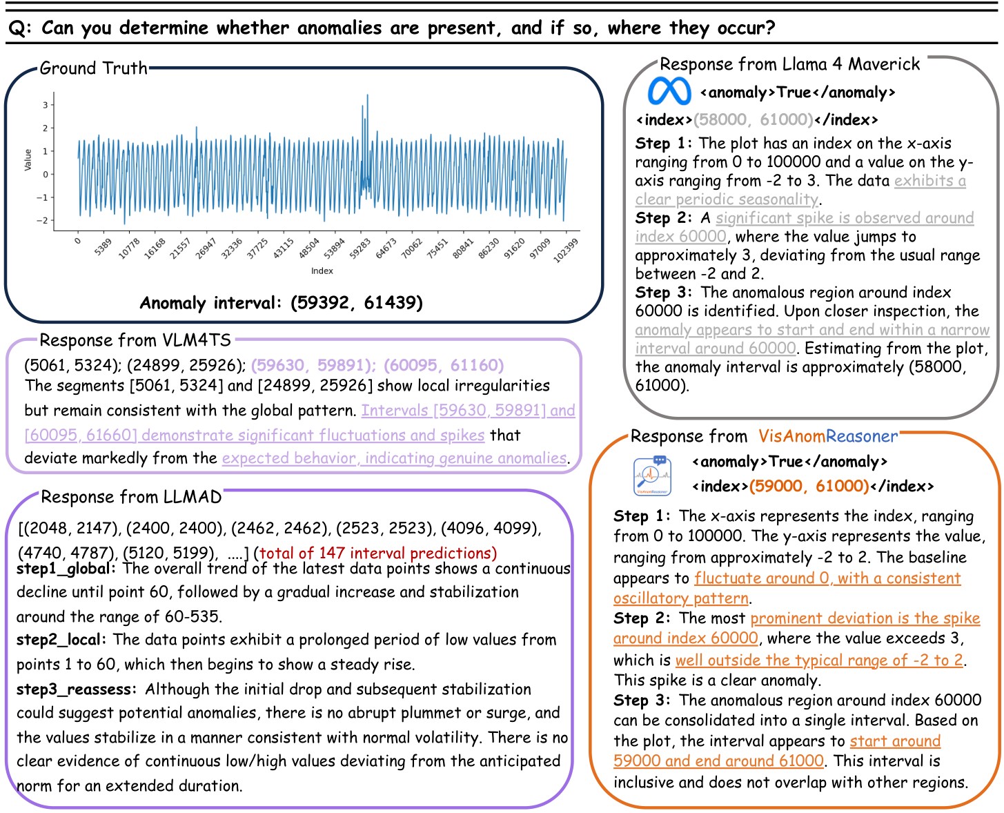
Table 7 checks that the result is not only against VLM and classical detector baselines. The reported deep-learning TSAD baselines remain far below VisAnomReasoner on interval-level F1.
| Model | TP | FP | FN | Precision | Recall | F1 |
|---|---|---|---|---|---|---|
| CS-LSTM | 175 | 556 | 584 | 23.94 | 23.06 | 23.49 |
| Anomaly-Transformer | 86 | 551 | 673 | 13.50 | 11.33 | 12.32 |
| Image-Embedding-CAE | 211 | 466 | 471 | 31.17 | 30.94 | 31.05 |
| AE | 297 | 439 | 459 | 40.35 | 39.29 | 39.81 |
| CNN | 237 | 481 | 522 | 33.01 | 31.23 | 32.09 |
| LSTM | 209 | 525 | 550 | 28.47 | 27.54 | 28.00 |
| VisAnomReasoner (7B) | 576 | 223 | 183 | 72.09 | 75.88 | 73.94 |
Table 7. Comparison with deep-learning TSAD baselines. These baselines are not vision-language methods, but their poor interval-level scores strengthen the paper's argument that standard sequence models do not directly solve this benchmark.
Efficiency
The paper reports that VisAnomReasoner uses LoRA rather than full-model training, with 95,178,752 trainable parameters or 1.13 percent of the backbone. For inference, it reports 16.5 plus/minus 2.3 seconds per input series and says runtime is largely insensitive to sequence length because the model reads a rendered plot rather than raw tokens. VLM4TS is reported as much slower, up to 452.6 seconds per series, while GPT-4o prompting methods average 3.8 seconds but have high variance and cannot process sequences longer than 14K points.
Practical Takeaways
- The cleanest reusable idea is not a new detector head; it is the source pipeline: render long time series as plots, require parsable interval tags, and supervise explanations that explicitly mention axis values and visible deviations.
- The strongest evidence is in-domain VisAnomBench performance. The 7B model's false positives drop sharply relative to Qwen2.5-VL-7B, and the 3B model has the best boundary Overlap.
- The cross-benchmark TSB-AD-U result is promising because it keeps strong affiliation precision and F1, but it is still limited to the paper's fixed univariate subset.
- Explanation quality is plausible but not fully settled. The paper uses GPT-4o preference judging and qualitative examples; it does not provide a large human expert study or faithfulness test against hidden raw numerical causes.
- The method depends on visualization quality. If an anomaly is compressed, visually ambiguous, multivariate, or only visible through raw numeric transformations, the paper's plot-first formulation may fail.
- The "tiny but trusted" framing is supported for this benchmark family: a LoRA-tuned Qwen2.5-VL-7B beats much larger general VLMs on the reported metrics. It should not be read as proof that small VLMs are universally reliable anomaly detectors.